Swin Transformer: Hierarchical Vision Transformer using Shifted Windows 제3부

Relative position bias

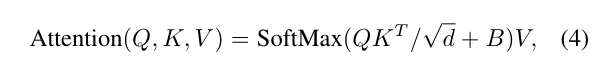
In computing self-attention, we follow [45, 1, 29, 30] by including a relative position bias B ∈ RM2 × M2 to each head in computing similarity:
자기 주의를 계산할 때 유사성을 계산할 때 각 헤드에 대한 상대 위치 편향 B ∈ RM2 × M2를 포함하여 [45, 1, 29, 30]을 따릅니다.

where Q, K, V ∈ R M 2 ×d are the query, key and value matrices; d is the query/key dimension, and M 2 is the number of patches in a window. Since the relative position along each axis lies in the range [−M + 1, M − 1], we parameterize a smaller-sized bias matrix ˆB ∈ R (2M −1)×(2M −1) , and values in B are taken from ˆB.
여기서 Q, K, V ∈ RM 2 × d는 쿼리, 키 및 값 행렬이며, d는 쿼리/키 차원이고, M2는 창의 패치 수입니다. 각 축을 따라 상대적인 위치가 [-M + 1, M - 1] 범위에 있기 때문에 더 작은 크기의 바이어스 행렬 matrix B r R (2M-1) × (2M-1)을 매개 변수화하고, B의 값은 bB에서 가져온다.

We observe significant improvements over counterparts without this bias term or that use absolute position embedding, as shown in Table 4. Further adding absolute position embedding to the input as in [19] drops performance slightly, thus it is not adopted in our implementation.
우리는 표 4에서와 같이 이 편향 항이 없거나 절대 위치 임베딩을 사용하는 대응물에 비해 상당한 개선을 관찰했습니다. [19]에서와 같이 입력에 절대 위치 임베딩을 추가로 추가하면 성능이 약간 떨어지므로 구현에서 채택되지 않았습니다.

The learnt relative position bias in pre-training can be also used to initialize a model for fine-tuning with a different window size through bi-cubic interpolation [19, 57].
사전 훈련에서 학습된 상대 위치 편향은 bi-cubic 보간을 통해 다른 창 크기로 미세 조정하기 위한 모델을 초기화하는 데 사용할 수도 있습니다[19, 57].

3.3. Architecture Variants

We build our base model, called Swin-B, to have of model size and computation complexity similar to ViTB/DeiT-B. We also introduce Swin-T, Swin-S and Swin-L, which are versions of about 0.25×, 0.5× and 2× the model size and computational complexity, respectively.
우리는 ViTB/DeiT-B와 유사한 모델 크기와 계산 복잡성을 갖도록 Swin-B라는 기본 모델을 구축합니다. 또한 Swin-T, Swin-S 및 Swin-L을 소개합니다. Swin-L은 각각 모델 크기와 계산 복잡성의 약 0.25배, 0.5배 및 2배의 버전입니다.

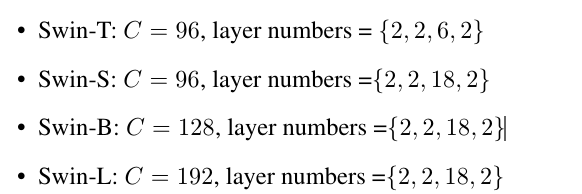
Note that the complexity of Swin-T and Swin-S are similar to those of ResNet-50 (DeiT-S) and ResNet-101, respectively. The window size is set to M = 7 by default. The query dimension of each head is d = 32, and the expansion layer of each MLP is α = 4, for all experiments. The architecture hyper-parameters of these model variants are:
Swin-T 및 Swin-S의 복잡성은 각각 ResNet-50(DeiT-S) 및 ResNet-101의 복잡성과 유사합니다. 창 크기는 기본적으로 M = 7로 설정됩니다. 모든 실험에서 각 헤드의 쿼리 차원은 d = 32이고 각 MLP의 확장 계층은 α = 4입니다. 이러한 모델 변형의 아키텍처 하이퍼 매개변수는 다음과 같습니다.

where C is the channel number of the hidden layers in the first stage. The model size, theoretical computational complexity (FLOPs), and throughput of the model variants for ImageNet image classification are listed in Table 1.
여기서 C는 첫 번째 단계에서 숨겨진 레이어의 채널 번호입니다. ImageNet 이미지 분류를 위한 모델 크기, 이론적 계산 복잡성(FLOP) 및 처리량은 표 1에 나열되어 있습니다.