TransFG: A Transformer Architecture for Fine-Grained Recognition 제3부
Experiments
In this section, we first introduce the detailed setup including datasets and training hyper-parameters. Quantitative analysis is then given followed by ablation studies. We further give qualitative analysis and visualization results to show the interpretability of our model.
이 섹션에서는 먼저 데이터 세트와 훈련 하이퍼 파라미터를 포함한 자세한 설정을 소개한다. 그런 다음 정량 분석 후 절제 연구가 제공됩니다. 또한 모델의 해석 가능성을 보여주기 위해 정성적 분석 및 시각화 결과를 제공한다.
Experiments Setup
Datasets.
We evaluate our proposed TransFG on five widely used fine-grained benchmarks, i.e., CUB-200-2011 (Wah et al. 2011), Stanford Cars (Krause et al. 2013), Stanford Dogs (Khosla et al. 2011), NABirds (Van Horn et al. 2015) and iNat2017 (Van Horn et al. 2018). We also exploit its usage in large-scale challenging fine-grained competitions.
Implementation details.
Unless stated otherwise, we implement TransFG as follows. First, we resize input images to 448 ∗ 448 except 304 ∗ 304 on iNat2017 for fair comparison (random cropping for training and center cropping for testing). We split image to patches of size 16 and the step size of sliding window is set to be 12. Thus the H, W, P, S in Eq 1 are 448, 448, 16, 12 respectively. The margin α in Eq 9 is set to be 0.4. We load intermediate weights from official ViT-B 16 model pretrained on ImageNet21k. The batch size is set to 16. SGD optimizer is employed with a momentum of 0.9. The learning rate is initialized as 0.03 except 0.003 for Stanford Dogs dataset and 0.01 for iNat2017 dataset. We adopt cosine annealing as the scheduler of optimizer.
달리 명시되지 않는 한, Trans를 구현합니다FG는 다음과 같다. 먼저, 공정한 비교를 위해 iNat2017에서 304 ∗ 304를 제외한 입력 이미지의 크기를 448 ∗ 448로 조정한다(훈련을 위한 무작위 자르기 및 테스트를 위한 센터 자르기). 이미지를 16 크기의 패치로 분할하고 슬라이딩 윈도우의 스텝 크기는 12로 설정합니다. 따라서 Eq 1의 H, W, P, S는 각각 448, 448, 16, 12이다. Eq 9의 마진α는 0.4로 설정된다. 우리는 ImageNet21k에서 사전 훈련된 공식 ViT-B 16 모델에서 중간 가중치를 로드한다. 배치 크기는 16으로 설정됩니다. SGD 최적화 도구는 0.9의 운동량으로 사용됩니다. 학습률은 Stanford Dogs 데이터 세트의 경우 0.003, iNat 2017 데이터 세트의 경우 0.01을 제외하고 0.03으로 초기화된다. 우리는 코사인 어닐링을 옵티마이저의 스케줄러로 채택한다.
Quantitative Analysis
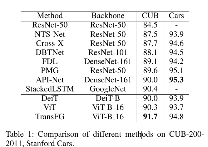
We compare our proposed method TransFG with state-ofthe-art works on above mentioned fine-grained datasets. The experiment results on CUB-200-2011 and Stanford Cars are shown in Table 1. From the results, we find that our method outperforms all previous methods on CUB dataset and achieve competitive performance on Stanford Cars.
우리는 제안된 방법 Trans를 비교한다위에서 언급한 세분화된 데이터 세트에 대한 최첨단 작업을 포함한 FG. CUB-200-2011 및 Stanford Cars에 대한 실험 결과는 표 1에 나와 있습니다. 결과로부터, 우리는 우리의 방법이 CUB 데이터 세트에서 이전의 모든 방법을 능가하고 스탠포드 자동차에서 경쟁력 있는 성능을 달성한다는 것을 발견했다.
To be specific, the third column of Table 1 shows the comparison results on CUB-200-2011. Compared to the best result StackedLSTM (Ge, Lin, and Yu 2019b) up to now, our TransFG achieves a 1.3% improvement on Top-1 Accuracy metric and 1.4% improvement compared to our base framework ViT (Dosovitskiy et al. 2020). Multiple ResNet-50 are adopted as multiple branches in (Ding et al. 2019) which greatly increases the complexity. It is also worth noting that StackLSTM is a very messy multi-stage training model which hampers the availability in practical use, while our TransFG maintains the simplicity.
구체적으로, 표 1의 세 번째 열은 Cub-200-2011의 비교 결과를 보여줍니다. 현재까지 최상의 결과 Stackedlstm (GE, LIN 및 YU 2019b)과 비교할 때, TransFG는 기본 프레임 워크 VIT (Dosovitskiy et al. 2020)에 비해 1.3% 개선을 달성하고 1.4% 개선을 달성합니다. 다중 RESNET-50은 복잡성을 크게 증가시키는 (Ding et al. 2019)에서 다수의 분기로 채택된다. 또한 STACKLSTM은 실질적인 사용으로 가용성을 방해하는 매우 지저분한 다단 훈련 모델이라는 점도 주목할 가치가 있습니다.