
SQL을 활용한 프로젝트 전에 연습용으로 Google Analytics Sample Dataset에서 인기 있는 노트북 몇개를 필사해보기로 했다. Top2 2개를 참고해서 한글로 번역하고, 시각화를 내가 편한 방식으로 일부 바꿔봤다.
Kaggle notebok 공유는 처음인데 벌써 감사히도 누군가 vote를 눌러줬다. 초심자를 위한 고수들의 따뜻한 칭찬 같은 느낌.

Intro
분석 목표
- Google Merchandise Store의 구글 애널리틱스 데이터를 SQL(BigQuery)을 활용하여 분석한다.
- SQL쿼리문을 활용해서 데이터셋에서 원하는 데이터를 추출하고 Python라이브러리를 활용한 시각화로 EDA를 진행한다.
데이터셋
- 원본 데이터 : Google Analytics Sample
- 데이터가 수집된 사이트 : Google Merchandise Store
- 기간 : 2016년 8월 1일 ~ 2017년 8월 1일
- 요약 (구글 애널리틱스에서 제공되는 데이터 종류) :
- 트래픽 소스 데이터: 웹사이트 방문자의 출처에 대한 정보(자연 트래픽, 유료 검색 트래픽, 디스플레이 트래픽 등)
- 콘텐츠 데이터: 사이트에서 사용자의 행동에 대한 정보(방문자가 보는 페이지의 URL, 콘텐츠와 상호 작용하는 방식 등)
- 거래 데이터: 웹사이트에서 발생하는 거래에 관한 정보.
- etc.
참고한 노트북
- PAUL MOONEY - How to Query the Google Analytics Sample Dataset
- DILLON MYRICK - SQL | EDA of Google Analytics Data
- 정우일 블로그 - Python BigQuery 연동하기
1. 라이브러리 로드
# BigQuery
from google.cloud import bigquery

# viz libraries
import pandas as pd
import seaborn as sns
import matplotlib.pyplot as plt
from plotly.offline import init_notebook_mode, iplot
import plotly.graph_objs as go
import plotly.express as px
from plotly.subplots import make_subplots

# viz settings
%matplotlib inline
sns.set()
init_notebook_mode(connected=True)
2. 데이터 연결, 확인
kaggle kernel에서 빅쿼리 데이터셋을 연결할 수 있다.
# Client 객체 생성
client = bigquery.Client()

# 데이터셋 참조경로(reference) 설정
# Kaggle커널에서는 bq_helper를 대신 사용할 수도 있다.
dataset_ref = client.dataset('google_analytics_sample', project='bigquery-public-data')

# 해당 경로로부터 데이터셋 추출
dataset = client.get_dataset(dataset_ref)
데이터셋은 여러 개의 테이블로 구성되어 있다.
# 데이터셋을 테이블 단위로 보기
tables = list(client.list_tables(dataset))
table_names = sorted([t.table_id for t in tables])

# 테이블 단위로 간단한 정보 확인
print(f"""table 개수 : {len(tables)}
tables : {", ".join(table_names[:3])}, ...
date 범위 : {table_names[0][-8:]} ~ {table_names[-1][-8:]}""")
데이터셋에서 하나의 테이블을 추출하고 일부를 출력해서 컬럼 정보와 구성을 확인할 수 있다.
# 테이블 경로 생성
table_ref_temp = dataset_ref.table(table_names[0])

# 테이블 가져오기
table_temp = client.get_table(table_ref_temp)

# 컬럼 확인
client.list_rows(table_temp, max_results=5).to_dataframe()| visitorId | visitNumber | visitId | visitStartTime | date | totals | trafficSource | device | geoNetwork | customDimensions | hits | fullVisitorId | userId | channelGrouping | socialEngagementType |
|---|---|---|---|---|---|---|---|---|---|---|---|---|---|---|
| NaN | 1 | 1470046245 | 1470046245 | 20160801 | {'visits': 1, 'hits': 24, 'pageviews': 17, ... | {'referralPath': None, 'campaign': '(not set)'... | {'browser': 'Firefox', 'browserVersion': 'not ... | {'continent': 'Europe', 'subContinent': 'Weste... | [{'index': 4, 'value': 'EMEA'}] | [{'hitNumber': 1, 'time': 0, 'hour': 3, 'minut... | 895954260133011192 | None | Organic Search | Not Socially Engaged |
| NaN | 1 | 1470084717 | 1470084717 | 20160801 | {'visits': 1, 'hits': 24, 'pageviews': 18, ... | {'referralPath': None, 'campaign': '(not set)'... | {'browser': 'Internet Explorer', 'browserVersi... | {'continent': 'Americas', 'subContinent': 'Nor... | [{'index': 4, 'value': 'North America'}] | [{'hitNumber': 1, 'time': 0, 'hour': 13, 'minu... | 0288478011259077136 | None | Direct | Not Socially Engaged |
| NaN | 3 | 1470078988 | 1470078988 | 20160801 | {'visits': 1, 'hits': 27, 'pageviews': 17, ... | {'referralPath': None, 'campaign': '(not set)'... | {'browser': 'Safari', 'browserVersion': 'not a... | {'continent': 'Americas', 'subContinent': 'Nor... | [{'index': 4, 'value': 'North America'}] | [{'hitNumber': 1, 'time': 0, 'hour': 12, 'minu... | 6440789996634275026 | None | Organic Search | Not Socially Engaged |
| NaN | 4 | 1470075581 | 1470075581 | 20160801 | {'visits': 1, 'hits': 27, 'pageviews': 19, ... | {'referralPath': '/', 'campaign': '(not set)',... | {'browser': 'Chrome', 'browserVersion': 'not a... | {'continent': 'Americas', 'subContinent': 'Nor... | [{'index': 4, 'value': 'North America'}] | [{'hitNumber': 1, 'time': 0, 'hour': 11, 'minu... | 8520115029387302083 | None | Referral | Not Socially Engaged |
| NaN | 30 | 1470099026 | 1470099026 | 20160801 | {'visits': 1, 'hits': 27, 'pageviews': 17, ... | {'referralPath': None, 'campaign': '(not set)'... | {'browser': 'Chrome', 'browserVersion': 'not a... | {'continent': 'Americas', 'subContinent': 'Nor... | [{'index': 4, 'value': 'North America'}] | [{'hitNumber': 1, 'time': 0, 'hour': 17, 'minu... | 6792260745822342947 | None | Organic Search | Not Socially Engaged |
결과 : Google Analytics 데이터로 totals, trafficSource, device, geoNetwork, customDimensions, hits 컬럼은 nested data(하나의 스키마 안에 여러 개의 데이터가 중첩된 구조)인 것을 확인할 수 있습니다.
아래는 위의 nested data 컬럼 내에 어떤 데이터가 포함되었는지 확인하는 과정입니다.
def format_schema_field(schema_field, indent=0):
    """
    빅쿼리 스키마의 (중첩된 구조 내부까지) 필드 이름과 데이터 타입을 출력하는 함수
    """

    indent_str = "  " * indent
    field_info = f"{indent_str}{schema_field.name} ({schema_field.field_type})"

    if schema_field.mode != "NULLABLE":
        field_info += f" - {schema_field.mode}"

    if schema_field.description:
        field_info += f" - {schema_field.description}"

    nested_indent = indent + 2
    if schema_field.field_type == "RECORD":
        for sub_field in schema_field.fields:
            field_info += "\n" + format_schema_field(sub_field, nested_indent)

    return field_info

# Display schemas
print("SCHEMA field for the 'totals' column:\n")
print(format_schema_field(table_temp.schema[5]))
print()

print("\nSCHEMA field for the 'trafficSource' column:\n")
print(format_schema_field(table_temp.schema[6]))
print()

print("\nSCHEMA field for the 'device' column:\n")
print(format_schema_field(table_temp.schema[7]))
print()

print("\nSCHEMA field for the 'geoNetwork' column:\n")
print(format_schema_field(table_temp.schema[8]))
print()

print("\nSCHEMA field for the 'customDimensions' column:\n")
print(format_schema_field(table_temp.schema[9]))
print()

print("\nSCHEMA field for the 'hits' column:\n")
print(format_schema_field(table_temp.schema[10]))
3. 분석 목표 설정
데이터셋의 구조와 대략적인 내용을 파악했습니다. 이제 활용 가능한 데이터의 종류를 알고 있기 때문에 어떤 데이터를 분석해서 어떤 정보를 얻을 것인지 구체적인 목표 설정이 가능합니다.
- 이탈률/종료율 분석 : 가장 많은 방문이 일어나는 인기 페이지, 이탈율/종료율이 높은 페이지?
- 브라우저/기기 분석 : 가장 많이 사용되는 브라우저/기기 종류, 이탈율이 높은 브라우저/기기?
- 사이트 트래픽 분석 : 사이트 트래픽 종류별 품질?
- 퍼널(전환 경로) 분석 : 고객 전환 경로 확인, 특정 전환단계에서 병목현상이 존재하는지?
- 상품 카테고리별 수요 분석 : 가장 잘 팔리는 카테고리와 예상 수요?
4. EDA with BigQuery
4-1. 이탈률/종료율 분석
방문수(views)
- 가장 많은 방문이 이뤄지는 랜딩페이지는 어디인가?
이탈률(bounce_rate)
- 이탈률 = 이탈수(totals.bounces) / 방문수(views)
- 이탈률이 높다는 것은 광고타겟설정, SEO, 페이지의 기능에 문제가 있을 수 있다는 의미한다.
- view기준 상위 10개 랜딩페이지의 방문수(view)와 이탈률(bounce_rate)를 확인했을 때
- bounce_rate가 낮은 경우 : apparel/men++s, bags (0.44, 0.45)
- bounce_rate가 높은 경우 : youtube, drinkware (0.56, 0.53)
# UNNEST(hits) : hits를 컬럼별로 분리시키기
# _TABLE_SUFIX : table 이름이 ~로 끝나는 경우
# hits.hitNumber=1 : 랜딩페이지로 한정

query = f"""
SELECT
    hits.page.pagePath AS landing_page,
    COUNT(*) AS views,
    SUM(totals.bounces)/COUNT(*) AS bounce_rate
FROM
    `bigquery-public-data.google_analytics_sample.ga_sessions_*`,
    UNNEST(hits) AS hits
WHERE
    _TABLE_SUFFIX BETWEEN '20160801' AND '20170801'  AND
    hits.type = 'PAGE'  AND
    hits.hitNumber=1
GROUP BY landing_page
ORDER BY 2 DESC
LIMIT 10
"""

result_bounce = client.query(query).result().to_dataframe()
result_bounce['label'] = result_bounce['landing_page'].str.split('/').str[-1]
result_bounce| index | landing_page | views | bounce_rate | label |
|---|---|---|---|---|
| 0 | /home | 612140 | 0.495475 | home |
| 1 | /google+redesign/shop+by+brand/youtube | 81512 | 0.562347 | youtube |
| 2 | /google+redesign/apparel/men++s/men++s+t+shirts | 20685 | 0.441141 | men++s+t+shirts |
| 3 | /signin.html | 16296 | 0.361622 | signin.html |
| 4 | /google+redesign/apparel/mens/mens+t+shirts | 12691 | 0.475061 | mens+t+shirts |
| 5 | /basket.html | 9431 | 0.454565 | basket.html |
| 6 | /google+redesign/drinkware | 8833 | 0.533794 | drinkware |
| 7 | /google+redesign/bags | 8608 | 0.451208 | bags |
| 8 | /google+redesign/apparel/men++s/men++s+outerwear | 6345 | 0.432782 | men++s+outerwear |
| 9 | /google+redesign/apparel | 6326 | 0.448150 | apparel |
종료율(exit_rate)
- 종료율 = 종료수(totals.bounces) / 방문수(views)
- 위에서 이탈률(bounce_rate)을 확인했던 페이지의 종료율(exit_rate)를 확인했을 떄
- bounce_rate이 높았던 youtube,drinkware 페이지는 exit_rate도 상대적으로 높다.
- bounce_rate이 낮았던 apparel/men++s 관련 페이지의 exit_rate가 다른 페이지보다 상대적으로 높다.
query = f"""
SELECT
    hits.page.pagePath as page,
    COUNT(*) AS views,
    SUM(totals.bounces)/COUNT(*) AS exit_rate
FROM
    `bigquery-public-data.google_analytics_sample.ga_sessions_*`,
    UNNEST(hits) AS hits
WHERE
    _TABLE_SUFFIX BETWEEN '20160801' AND '20170801'  AND
    hits.type='PAGE'
GROUP BY 1
ORDER BY 2 desc
LIMIT 10
"""

result_exit = client.query(query).result().to_dataframe()
result_exit['label'] = result_exit['page'].str.split('/').str[-1]
result_exit| index | page | views | exit_rate | label |
|---|---|---|---|---|
| 0 | /home | 981285 | 0.309920 | home |
| 1 | /basket.html | 209360 | 0.020524 | basket.html |
| 2 | /google+redesign/shop+by+brand/youtube | 145026 | 0.316198 | youtube |
| 3 | /signin.html | 101299 | 0.058322 | signin.html |
| 4 | /store.html | 93551 | 0.025505 | store.html |
| 5 | /google+redesign/apparel/men++s/men++s+t+shirts | 67471 | 0.135392 | men++s+t+shirts |
| 6 | /asearch.html | 62380 | 0.031677 | asearch.html |
| 7 | /google+redesign/electronics | 56839 | 0.047116 | electronics |
| 8 | /google+redesign/apparel | 56552 | 0.050272 | apparel |
| 9 | /google+redesign/bags | 53686 | 0.072458 | bags |
이탈률과 종료율 시각화
위에서 이탈률(bounce_rate)을 확인했던 페이지의 종료율(exit_rate)를 확인했을 떄
- bounce_rate이 높았던 youtube,drinkware 페이지는 exit_rate도 상대적으로 높다.
- bounce_rate이 낮았던 apparel/men++s 관련 페이지의 exit_rate가 다른 페이지보다 상대적으로 높다.
# 이탈률 시각화
px.bar(result_bounce.sort_values(by='bounce_rate'), x='bounce_rate', y='label',
      width=800, height=400, title='Top10 랜딩페이지의 이탈률(Bounce Rate)')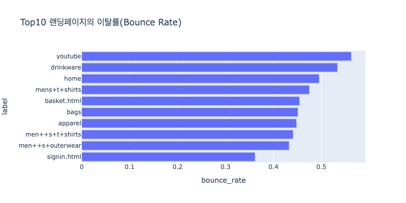
# 종료율 시각화
px.bar(result_exit.sort_values(by='exit_rate'), x='exit_rate', y='label',
      width=800, height=400, title='Top10 방문페이지의 종료율(Exit Rate)')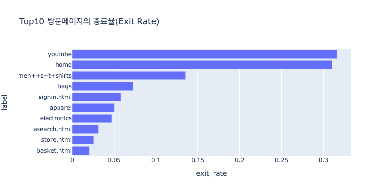
Insight :
- 장바구니(basket)와 로그인(signin)페이지가 Top10 랜딩페이지에 속한다.
- 재방문 고객이 많은 것을 알 수 있다.
- Top10 랜딩페이지 중 3가지 품목이 남성의류(Men's Apperal)에 해당한다.
- 해당 카테고리가 인기 품목이거나, 남성 고객이 주사용층일 수 있다.
- Youtube brand 상품 페이지는 랜딩과 방문 모두 1위인 페이지만 동시에 종료율과 이탈률도 높다.
- 검색어 설정이나 광고에서 모호한 문구로 고객들에게 혼동을 주고 있을 수 있다.
- (ex. 해당 페이지는 Youtube브랜드의 상품을 판매하는 페이지이지만 유튜버 콜라보 상품, 유튜브 컨텐츠로 유명한 상품, 유튜브 촬영을 위한 상품 등을 찾는 고객이 유입된 것이 아닐까?)
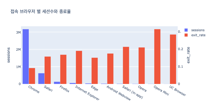
4-2. 브라우저/기기 분석
세션별 접속한 브라우저와 기기 정보를 확인하면 호환성 문제를 확인할 수 있다.
# 쿼리문
query = f"""
SELECT
    device.Browser AS browser,
    COUNT(*) AS sessions,
    SUM(totals.bounces)/COUNT(*) AS exit_rate
FROM
    `bigquery-public-data.google_analytics_sample.ga_sessions_*`,
    UNNEST(hits) AS hits
WHERE
    _TABLE_SUFFIX BETWEEN '20160801' AND '20170801'
GROUP BY 1
ORDER BY 2 desc
LIMIT 10
"""
result_browser = client.query(query).result().to_dataframe()
display(result_browser)


# 발견한 사실
print(f"""브라우저 : 접속 브라우저 별 세션수(session)와 종료율(exit_rate)를 확인했을 때
- Chrome 이 다른 브라우저에 비해 6% 이상 exit_rate이 낮다.""")


# 시각화
fig = go.Figure(
    data = [
        go.Bar(x=result_browser['browser'], y=result_browser['sessions'],
               yaxis='y', offsetgroup=1, name='sessions'),
        go.Bar(x=result_browser['browser'], y=result_browser['exit_rate'],
               yaxis='y2', offsetgroup=2, name='exit_rate')
    ],
    layout = {
        'yaxis' : {'title' : 'sessions'},
        'yaxis2' : {'title' : 'exit_rate', 'overlaying': 'y', 'side': 'right'}
    },
)

fig.update_layout(
    barmode='group', width=800, height=400, title="접속 브라우저 별 세션수와 종료율"
)
fig.show()| index | browser | sessions | exit_rate |
|---|---|---|---|
| 0 | Chrome | 3197849 | 0.091878 |
| 1 | Safari | 629906 | 0.157622 |
| 2 | Firefox | 133880 | 0.168195 |
| 3 | Internet Explorer | 62405 | 0.190369 |
| 4 | Edge | 38063 | 0.150934 |
| 5 | Android Webview | 25979 | 0.174872 |
| 6 | Safari (in-app) | 19037 | 0.213532 |
| 7 | Opera | 15439 | 0.209988 |
| 8 | Opera Mini | 12767 | 0.314639 |
| 9 | UC Browser | 5807 | 0.283968 |
기기
# 쿼리문
query = f"""
SELECT
    device.deviceCategory AS device,
    COUNT(*) AS sessions,
    SUM(totals.bounces)/COUNT(*) AS exit_rate
FROM
    `bigquery-public-data.google_analytics_sample.ga_sessions_*`,
    UNNEST(hits) AS hits
WHERE
    _TABLE_SUFFIX BETWEEN '20160801' AND '20170801'
GROUP BY 1
ORDER BY 2 desc
LIMIT 10
"""
result_device = client.query(query).result().to_dataframe()
display(result_device)


# 발견한 사실
print(f"""기기 : 접속 기기 별 세션수(session)와 종료율(exit_rate)을 확인했을 때
- desktop을 사용한 방문이 가장 많다.
- mobile의 종료율이 3% 정도 더 높다.""")


# 시각화
fig = go.Figure(
    data = [
        go.Bar(x=result_device['device'], y=result_device['sessions'],
               yaxis='y', offsetgroup=1, name='sessions'),
        go.Bar(x=result_device['device'], y=result_device['exit_rate'],
               yaxis='y2', offsetgroup=2, name='exit_rate')
    ],
    layout = {
        'yaxis' : {'title' : 'sessions'},
        'yaxis2' : {'title' : 'exit_rate', 'overlaying': 'y', 'side': 'right'}
    },
)

fig.update_layout(
    barmode='group', width=800, height=400, title="접속 기기 별 세션수와 종료율"
)
fig.show()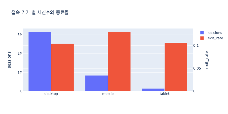
브라우저 + 기기
# 쿼리문
query = f"""
SELECT
    device.deviceCategory AS device,
    device.Browser AS browser,
COUNT(*) AS sessions,
    SUM(totals.bounces)/COUNT(*) AS exit_rate
FROM
    `bigquery-public-data.google_analytics_sample.ga_sessions_*`,
    UNNEST(hits) AS hits
WHERE
    _TABLE_SUFFIX BETWEEN '20160801' AND '20170801'
GROUP BY 1, 2
ORDER BY 3 desc
LIMIT 20
"""
result_browser_device = client.query(query).result().to_dataframe()
result_browser_device['browser_device'] = (
    result_browser_device["browser"].astype(str) + "-" + result_browser_device["device"].astype(str)
)
result_browser_device = result_browser_device.sort_values(by=['browser', 'device'])

# 발견한 사실
print(f"""앞에서 확인한
- Chrome 브라우저(exit_rate이 상대적으로 낮았음) 중에서도 mobile기기의 경우 desktop보다 exit_rate이 4% 더 높았다.
- desktop safari를 사용한 경우 exit_rate이 다른 기기-브라우저에 비해 높다.""")


# 시각화
fig = go.Figure(
    data = [
        go.Bar(x=result_browser_device['browser_device'], y=result_browser_device['sessions'],
               yaxis='y', offsetgroup=1, name='sessions'),
        go.Bar(x=result_browser_device['browser_device'], y=result_browser_device['exit_rate'],
               yaxis='y2', offsetgroup=2, name='exit_rate')
    ],
    layout = {
        'yaxis' : {'title' : 'sessions'},
        'yaxis2' : {'title' : 'exit_rate', 'overlaying': 'y', 'side': 'right'}
    },
)

fig.update_layout(
    barmode='group', width=800, height=400, title="접속 브라우저/기기 별 세션수와 종료율"
)
fig.show()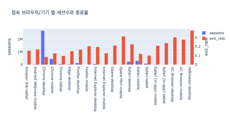
Insight :
- 해당 사이트는 주로 Chrome브라우저, Desktop기기에 최적화되어 있다.
- mobile기기의 이탈률이 desktop, tablet보다 더 높다.
- 최적화된 환경을 제공하고 있는지 확인해보고, 그렇지 않다면 mobile은 전체 session의 20% 정도를 차지하고 있으므로 개선이 필요할 수 있다.
- 상품 구경은 mobile로 하고 실제 최종 결제는 descktop에서 이뤄지고 있을 수도 있다. Chek out 페이지에 접속하는 브라우저/기기도 다시 살펴볼 필요가 있다.
4-3. 사이트 트래픽 소스 분석
- 전환율 : 전체 세션 중 완료된 트랜잭션의 비율
- 전환율(conversion_rate) = 트랜잭션수(trancations)/세션수(sessions)
Google Analytics에서 사용되는 각 트래픽 소스
- None (Direct): 사용자가 웹사이트에 직접 주소를 입력하거나,즐겨찾기를 통해 접속한 경우
- Referral: 다른 웹사이트에서 사용자가 클릭한 링크를 통해 웹사이트로 유입된 트래픽(ex.소셜 미디어 공유)
- Affiliate: 제휴사 또는 제휴 프로그램을 통해 유입된 트래픽
- Organic (Organic Search): 검색 엔진에서 검색 결과 페이지를 통해 유입된 트래픽입니다.
- CPC (Cost Per Click): 광고를 클릭하는 데에 비용이 지불된 트래픽
- CPM (Cost Per Mille): 광고 노출 횟수에 따른 비용을 기반으로 하는 트래픽
# 쿼리문
query = """
SELECT
    trafficSource.medium AS medium,
    count(*) AS sessions,
    SUM(totals.bounces)/COUNT(*) AS exit_rate,
    SUM(totals.transactions) AS transactions,
    SUM(totals.totalTransactionRevenue)/1000000 AS total_revenue,
    SUM(totals.transactions)/COUNT(*) AS conversion_rate
FROM
    `bigquery-public-data.google_analytics_sample.ga_sessions_*`,
    UNNEST(hits) AS hits
WHERE
    _TABLE_SUFFIX BETWEEN '20160801' AND '20170801'
GROUP BY 1
ORDER BY 2 desc
"""
result_traffic = client.query(query).result().to_dataframe()
display(result_traffic.head(10))


# 시각화
fig = go.Figure(
    data = [
        go.Bar(x=result_traffic['medium'], y=result_traffic['total_revenue'],
               yaxis='y', offsetgroup=1, name='total_revenue'),
        go.Bar(x=result_traffic['medium'], y=result_traffic['conversion_rate'],
               yaxis='y2', offsetgroup=2, name='conversion_rate')
    ],
    layout = {
        'yaxis' : {'title' : 'sessions'},
        'yaxis2' : {'title' : 'exit_rate', 'overlaying': 'y', 'side': 'right'}
    },
)

fig.update_layout(
    barmode='group', width=800, height=400, title="트래픽 소스별 매출액과 전환율"
)
fig.show()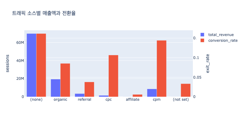
Insight :
- organic 트래픽이 많은 비중을 차지하지만
- 광고로 인한 유입(cpc, cpm)에서 전환율(conversion rate)이 다른 소스에 비해서 높다.
4-4. 퍼널(전환 경로) 분석
(Conversion path)
(Bottlenecks)
전환과정중 고객들이 이탈하는 곳 파악하기
hits.eCommerceAction.action_type
query = f"""
SELECT
    CASE
        WHEN hits.eCommerceAction.action_type = '1' THEN 'Click through of procut lists'
        WHEN hits.eCommerceAction.action_type = '2' THEN 'Product detail views'
        WHEN hits.eCommerceAction.action_type = '5' THEN 'Check out'
        WHEN hits.eCommerceAction.action_type = '6' THEN 'Completed purchase'
    END AS action,
    COUNT(fullVisitorID) AS users
FROM
    `bigquery-public-data.google_analytics_sample.ga_sessions_*`,
    UNNEST(hits) AS hits,
    UNNEST(hits.product) AS product
WHERE
    _TABLE_SUFFIX BETWEEN '20160801' AND '20170801'  AND
    (
    hits.eCommerceAction.action_type != '0'  AND
    hits.eCommerceAction.action_type != '3'  AND
    hits.eCommerceAction.action_type != '4'
    )
GROUP BY 1
ORDER BY 2 desc
"""
result = client.query(query).result().to_dataframe()
display(result.head(10))| index | action | users |
|---|---|---|
| 0 | Click through of product lists | 445760 |
| 1 | Product detail views | 362607 |
| 2 | Check out | 248936 |
| 3 | Completed purchase | 74457 |
# 퍼널 분석 시각화
funnel_graph = go.Figure(
    go.Funnel(
        x = result['users'],
        y = result['action'],
        textposition = 'inside',
        textinfo = 'value+percent initial'
    ),
    layout=go.Layout(height=400, width=800)
)
funnel_graph.update_layout(title_text = 'Google Merchandise Store 퍼널 분석')

funnel_graph.show()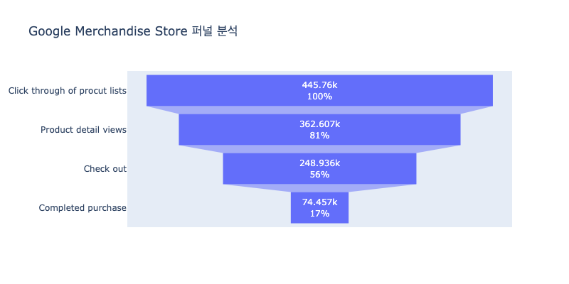
Insight :
- 상품 상세 페이지(Product detail views)에서 결제 페이지(Check out)로 넘어가는 비율은 68.7%로 높다.
- 그러나 결제 페이지(Check out)에서 실제 구매가 완료(Complete purchase)되는 비율은 29.9% 밖에 되지 않는다.
- 결제 페이지 ➔ 구매 완료 의 전환 과정에 문제가 있어 보인다.
- 상품 상세 페이지에서 보이는 금액과 결제 페이지에서 보이는 실제 예상 결제금액에 차이가 있는 것이 아닐까?
- 상품 상세 페이지에서 쿠폰 적용, 카드 결제할인, 멤버십 적립금 등의 할인 적용시의 금액 확인이 불편해서 Check out에서 확인하고 돌아가는 것이 아닐까?
- 상품 결제 수단이 한정적인가?
- 문제가 없는 것이라면 단순히 상품을 담아놓고 종료 후에 나중에 결제하는 고객이 많은 것이 아닐까? (위에서 basket, signin으로 바로 랜딩하는 고객이 많은 것을 확인했다.) 이렇게 결제를 완료하지 않고 보관만 하는 고객들을 결제로 유도할 전략(ex. "00분 안에 결제 시 오늘 출고" 문구)을 고려할 수 있다.
4-5. 상품 카테고리별 수요 분석
거래량과 매출
query = f"""
SELECT
    product.v2ProductCategory AS category,
    SUM(totals.transactions) AS transactions,
    SUM(totals.totalTransactionRevenue)/1000000 AS total_revenue
FROM
    `bigquery-public-data.google_analytics_sample.ga_sessions_*`,
    UNNEST(hits) AS hits,
    UNNEST(hits.product) AS product
WHERE
    _TABLE_SUFFIX BETWEEN '20160801' AND '20170801'
GROUP BY 1
ORDER BY 3 DESC
LIMIT 10
"""
cat_result = client.query(query).result().to_dataframe()

px.bar(cat_result.sort_values(by='total_revenue'),
       x='total_revenue', y='category',
       width=800, height=400, title="상품 카테고리별 매출액")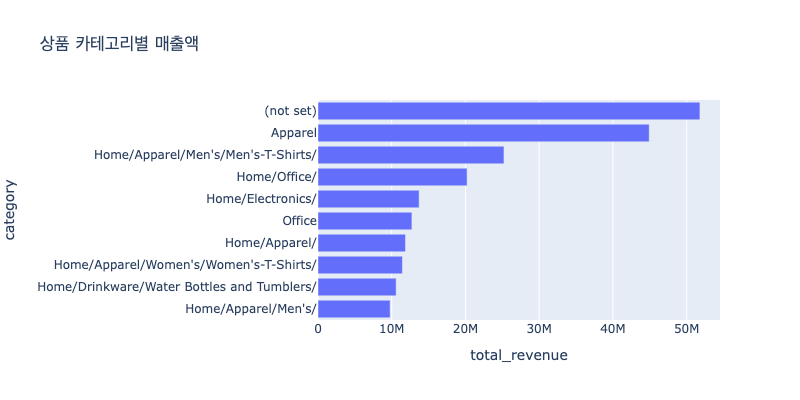
7일 이동평균 거래량
query = f"""
WITH
    daily_mens_tshirs_transactions AS
    (
    SELECT
        date,
        SUM(totals.transactions) AS transactions
    FROM
        `bigquery-public-data.google_analytics_sample.ga_sessions_*`,
        UNNEST(hits) AS hits,
        UNNEST(hits.product) AS product
    WHERE
        _TABLE_SUFFIX BETWEEN '20160801' AND '20170801'  AND
        product.v2ProductCategory = "Home/Apparel/Men's/Men's-T-Shirts/"
    GROUP BY 1
    ORDER BY 1
    )
SELECT
    date,
    AVG(transactions) OVER (
        ORDER BY date
        ROWS BETWEEN 3 PRECEDING AND 3 FOLLOWING
    ) AS avg_transactions
FROM
    daily_mens_tshirs_transactions

"""

result = client.query(query).result().to_dataframe()
result['date'] = pd.to_datetime(result['date'])

px.area(result, 'date', 'avg_transactions',
       title='<Men\'s T-Shirts> Conversions 7-Day Moving Average',
       height=400, width=800)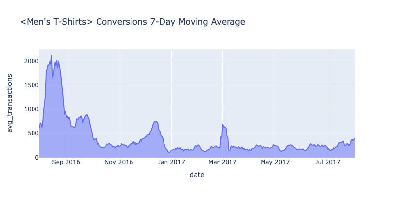
query = f"""
WITH
    daily_drinkware_transactions AS
    (
    SELECT
        date,
        SUM(totals.transactions) AS transactions
    FROM
        `bigquery-public-data.google_analytics_sample.ga_sessions_*`,
        UNNEST(hits) AS hits,
        UNNEST(hits.product) AS product
    WHERE
        _TABLE_SUFFIX BETWEEN '20160801' AND '20170801'  AND
        product.v2ProductCategory = "Home/Drinkware/Water Bottles and Tumblers/"
    GROUP BY 1
    ORDER BY 1
    )
SELECT
    date,
    AVG(transactions) OVER (
        ORDER BY date
        ROWS BETWEEN 3 PRECEDING AND 3 FOLLOWING
    ) AS avg_transactions
FROM
    daily_drinkware_transactions
"""

result = client.query(query).result().to_dataframe()
result['date'] = pd.to_datetime(result['date'])

px.area(result, 'date', 'avg_transactions',
       title='<drinkware> Conversions 7-Day Moving Average',
       height=400, width=800)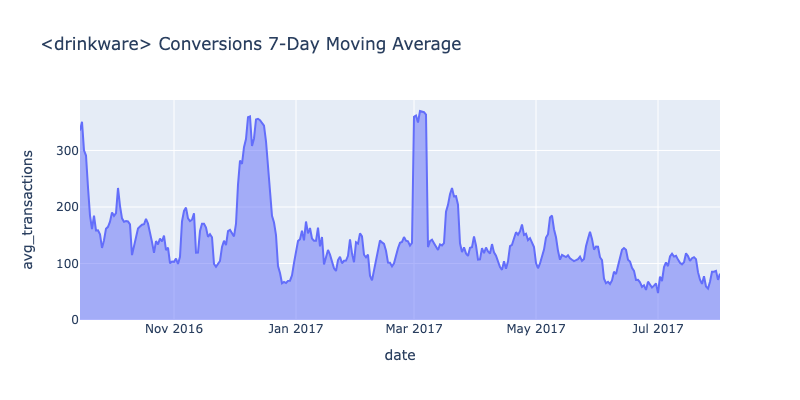
query = f"""
WITH
    daily_electronics_transactions AS
    (
    SELECT
        date,
        SUM(totals.transactions) AS transactions
    FROM
        `bigquery-public-data.google_analytics_sample.ga_sessions_*`,
        UNNEST(hits) AS hits,
        UNNEST(hits.product) AS product
    WHERE
        _TABLE_SUFFIX BETWEEN '20160801' AND '20170801'  AND
        product.v2ProductCategory = "Home/Electronics/"
    GROUP BY 1
    ORDER BY 1
    )
SELECT
    date,
    AVG(transactions) OVER (
        ORDER BY date
        ROWS BETWEEN 3 PRECEDING AND 3 FOLLOWING
    ) AS avg_transactions
FROM
    daily_electronics_transactions
"""

result = client.query(query).result().to_dataframe()
result['date'] = pd.to_datetime(result['date'])

px.area(result, 'date', 'avg_transactions',
       title='<Electronics> Conversions 7-Day Moving Average',
       height=400, width=800)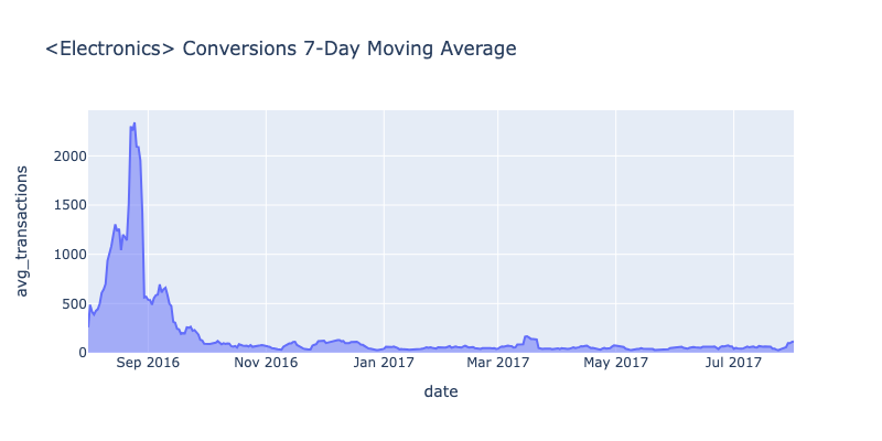
query = f"""
WITH
    daily_office_transactions AS
    (
    SELECT
        date,
        SUM(totals.transactions) AS transactions
    FROM
        `bigquery-public-data.google_analytics_sample.ga_sessions_*`,
        UNNEST(hits) AS hits,
        UNNEST(hits.product) AS product
    WHERE
        _TABLE_SUFFIX BETWEEN '20160801' AND '20170801'  AND
        product.v2ProductCategory = "Home/Office/"
    GROUP BY 1
    ORDER BY 1
    )
SELECT
    date,
    AVG(transactions) OVER (
        ORDER BY date
        ROWS BETWEEN 3 PRECEDING AND 3 FOLLOWING
    ) AS avg_transactions
FROM
    daily_office_transactions
"""

result = client.query(query).result().to_dataframe()
result['date'] = pd.to_datetime(result['date'])

px.area(result, 'date', 'avg_transactions',
       title='<office> Conversions 7-Day Moving Average',
       height=400, width=800)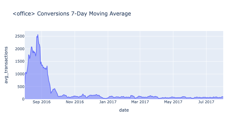
Insight :
- 2016년 (특히 8, 9월)의 매출이 그 이후의 매출에 비해 매우 높은 것을 확인할 수 있다. 왜 그럴까?
- Office, Electronics 상품은 위의 2016.08 ~ 09를 제외하면 매출의 변동이 적다.
- Drinkware 상품은 12월과 3월에 매출이 일시적으로 급증했다.
- Men's T-Shirts 상품은 12월, 3월, 8월에 매출이 증가했다.
상품 카테고리에 따라 매출이 일시적으로 증가한 것이 시계열(계절)적 특성인지 다른 해의 매출과 비교할 필요가 있다.
혹은 해당 기간에 광고, 세일 등이 이뤄졌는지 확인할 필요가 있다.
5. 분석결과(인사이트) 요약
위의 EDA를통해 몇 가지 눈여겨 볼 사실(Insight)을 발견했다. 이 인사이트를 기반으로 "왜 이런 현상이 발생했는지"에 대해서 더 구체적인 목표를 수립하고 세분화된 분석을 진행할 수 있다.
- 2016년 8월~9월의 매출 급증 이유
- 특정 품목 매출의 계절성 여부
- 결제 페이지의 문제 여부
- 결제를 미루고 재방문 시 구매하는 고객의 존재 여부
- Youtube 브랜드 상품 페이지의 검색어 최적화 여부
- 모바일에서의 사용 최적화 여부