Simcenter 사용법
1. 모델 파일 열기
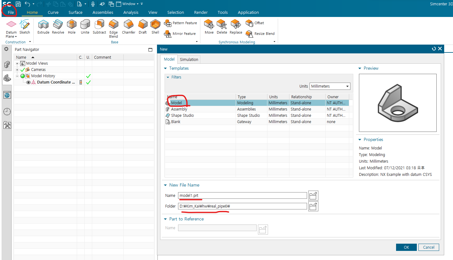
1-1) 새 prt 파일 생성
file - new 들어가서 파일명, 경로 설정하고, model 더블클릭
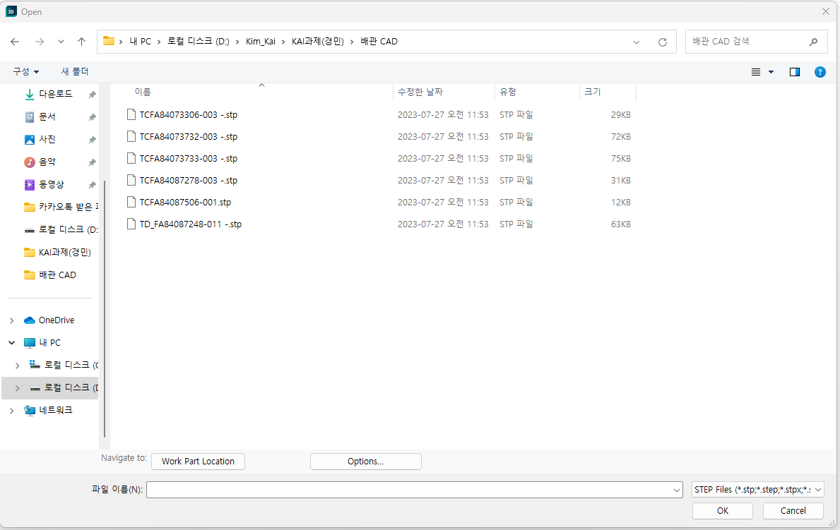
1-2) prt 파일 불러오기
그 후 file - open 눌러서 원하는 prt 파일 호출
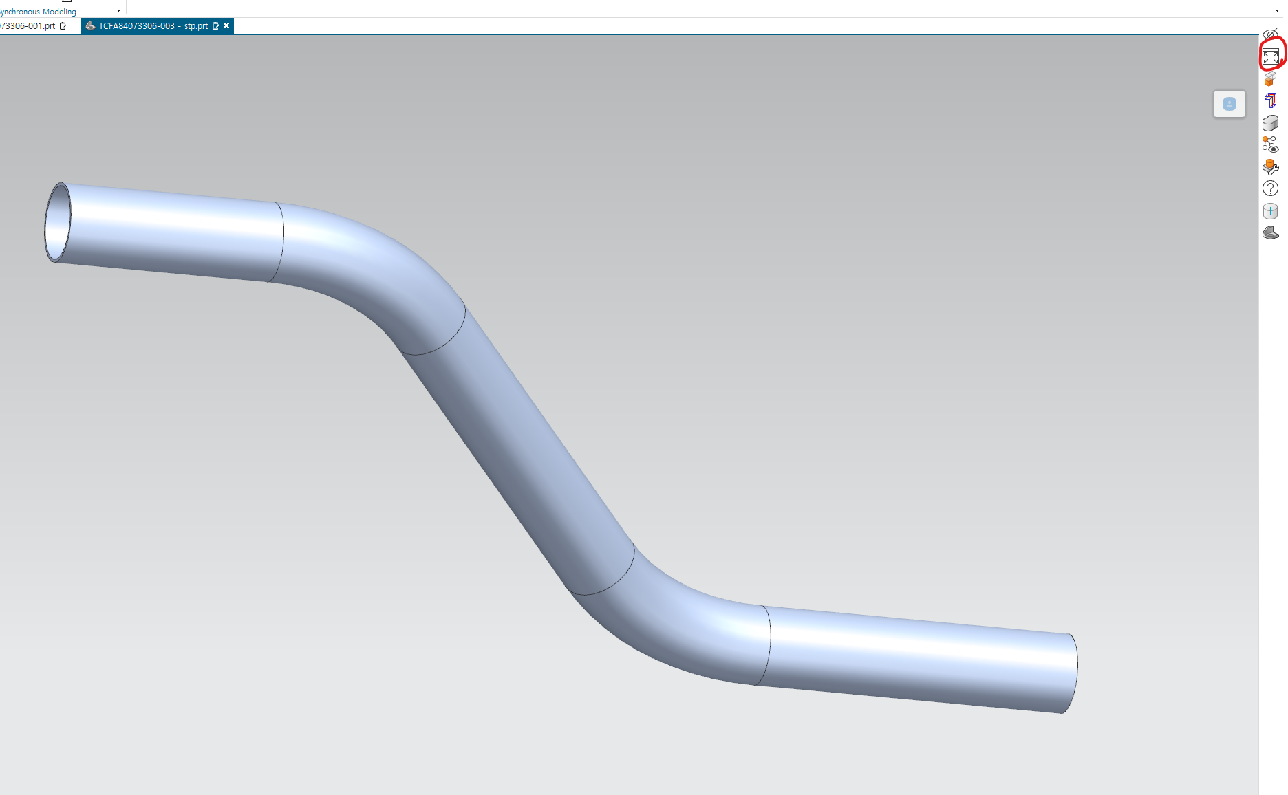
그리고 우측 툴바의 해당 버튼을 누르면, 모델링 형상이 가운데 정렬됨
1-3) prt 정렬
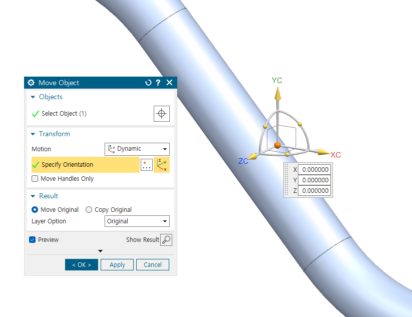
1. prt를 원점으로 이동 : menu -> edit->move object->dynamic
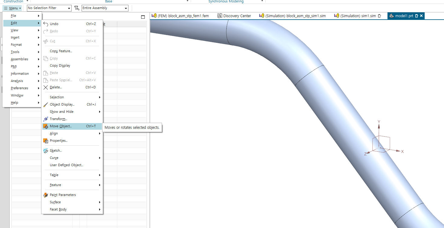
motion을 dynamic으로 설정 후, 원점을 더블 클릭하여, 지정
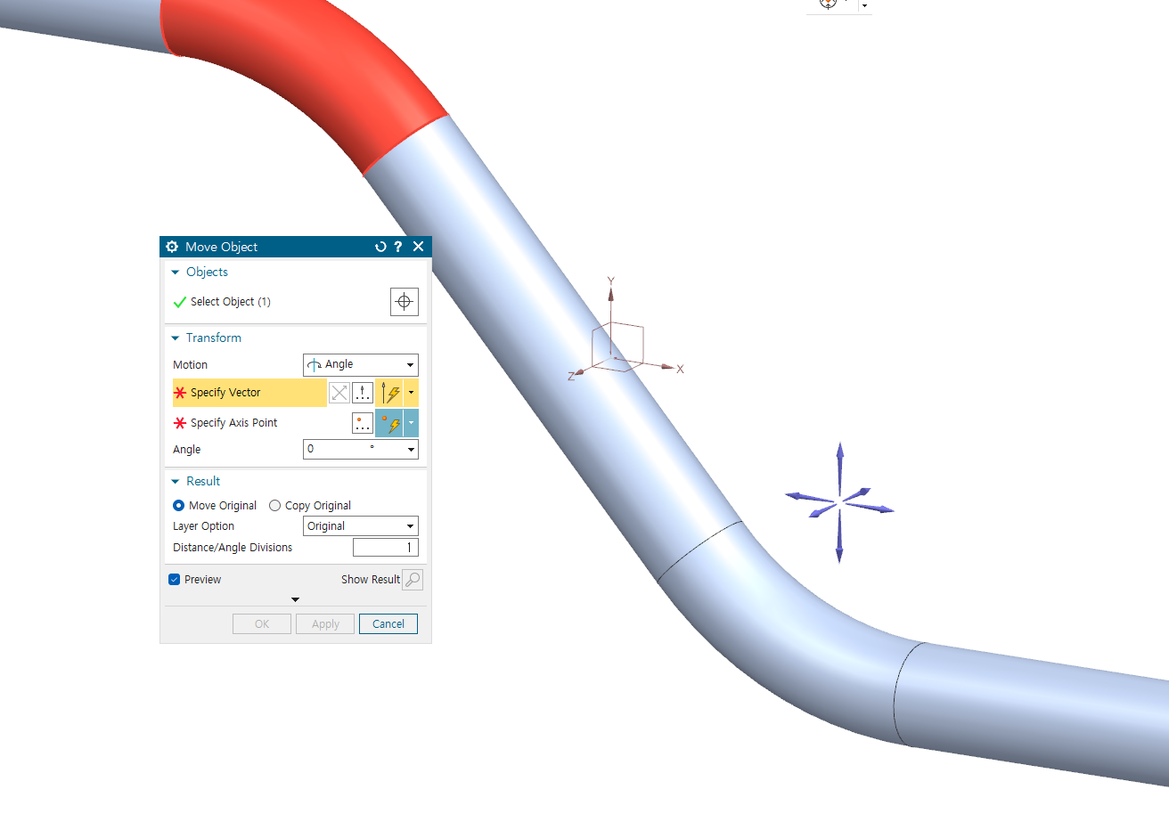
2. prt를 회전시키는 경우 : menu -> edit->move object->angle
2. mesh 생성
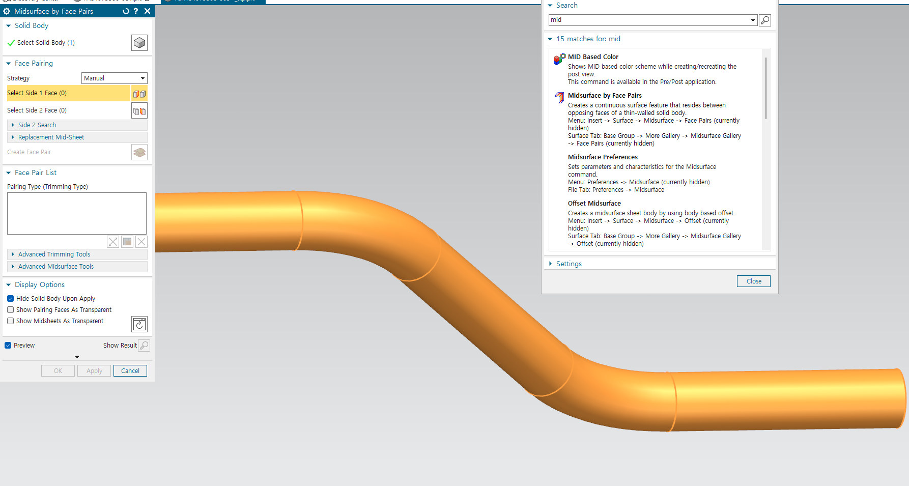
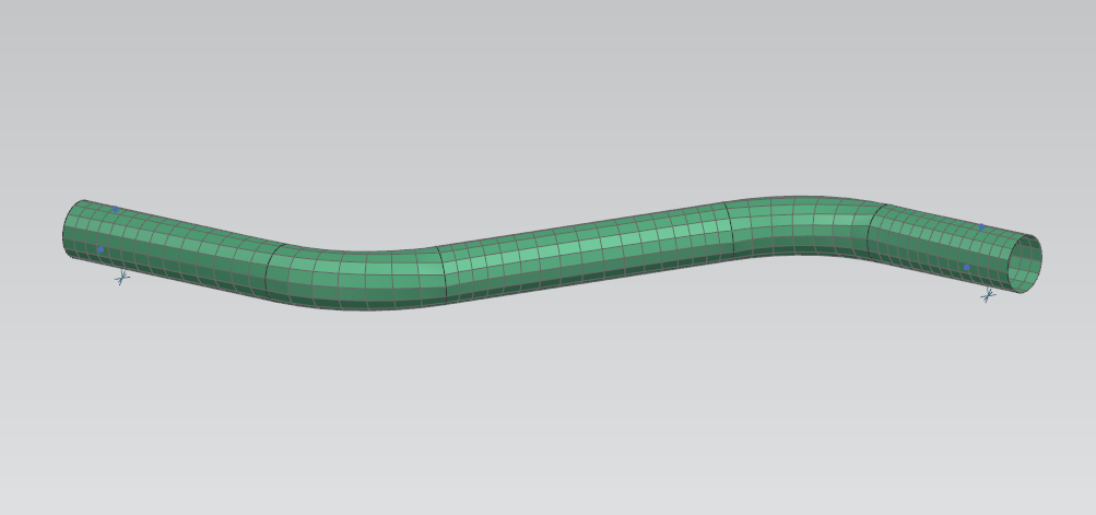
2-1) 파이프의 경우에는 midsurface로 shell로 만들기
돋보기 창에 mid surface 검색하고, midsurface by face pairs 버튼 선택
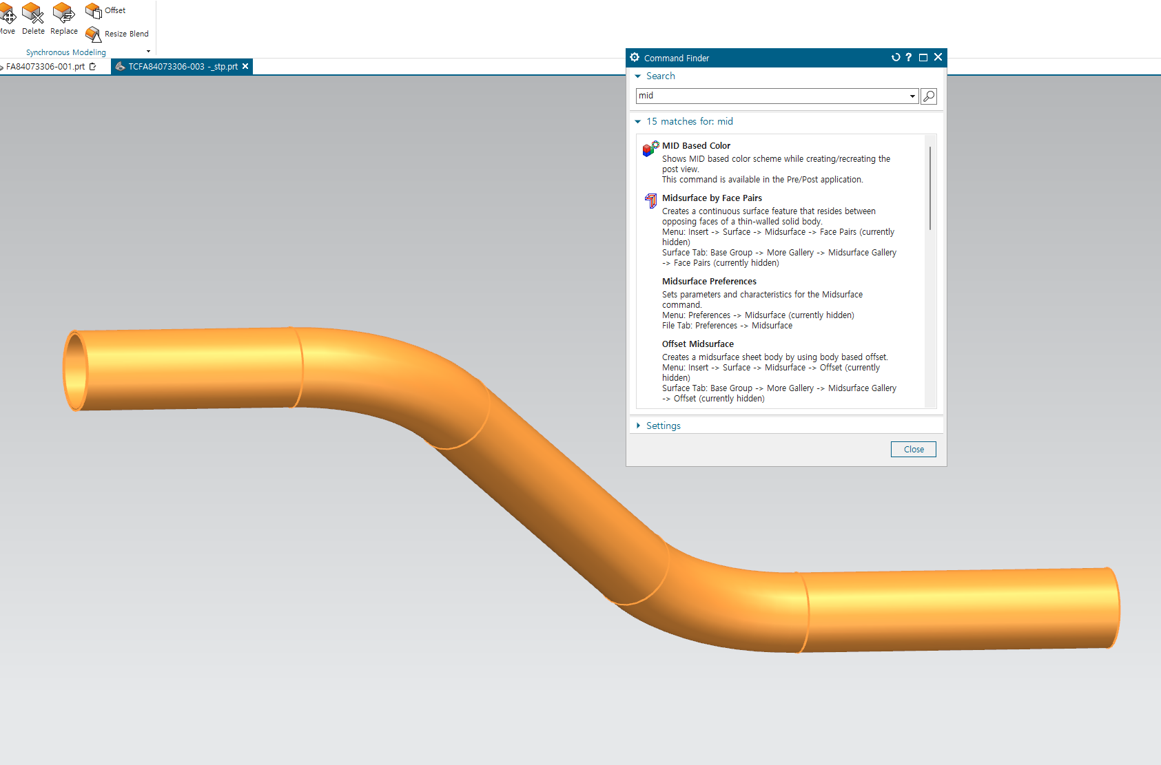
그리고 create face pair로 shell로 변환할 부피 선택
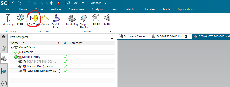
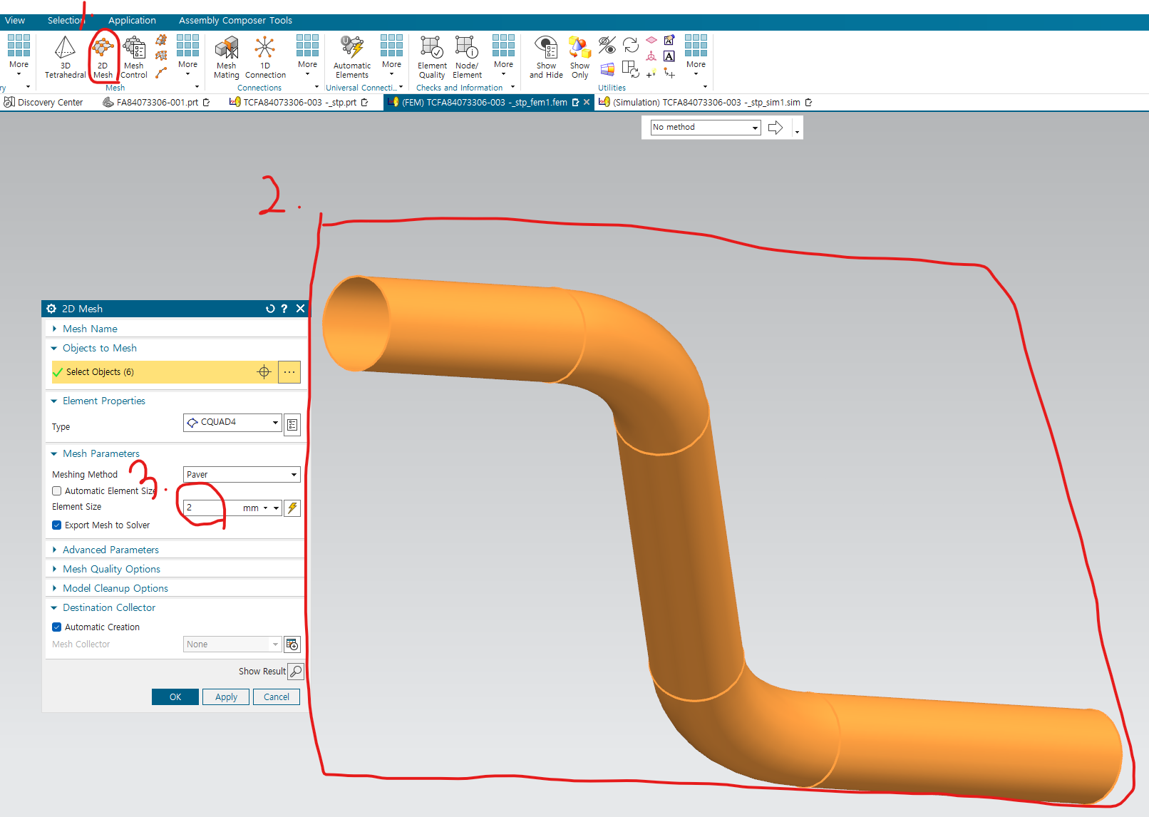
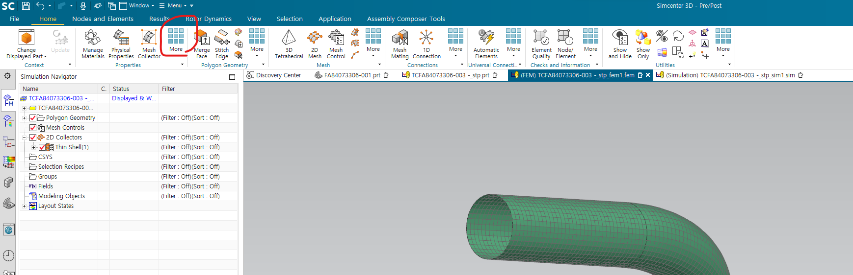
2-2) mesh 생성 - fem 생성
application tab의 pre/post 아이콘 클릭
상단의 new fem and simulation 선택
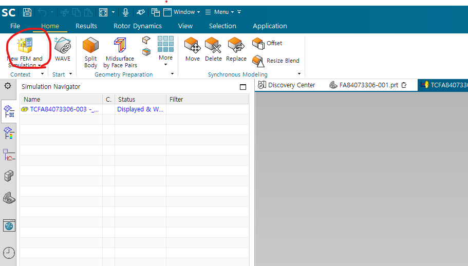
fem에 들어가서 mesh 생성 - 1. shell이므로 2D mesh 2. 드래그하여, mesh 생성하는 prt 선택 3. 원하는 element size 지정
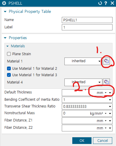
3. 물성치 및 두께 입력
thin shell 더블클릭 - 도구 모양 선택
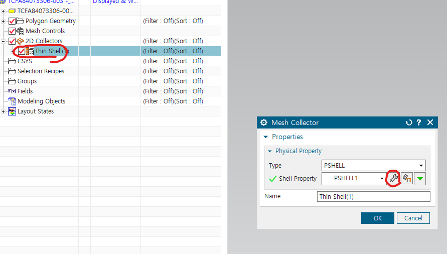
1번 버튼을 눌러서 원하는 물성치 입력 그리고 2번에 파이프 두께 입력
물성치 입력하는 또 다른 방법 - more의 assign material 선택
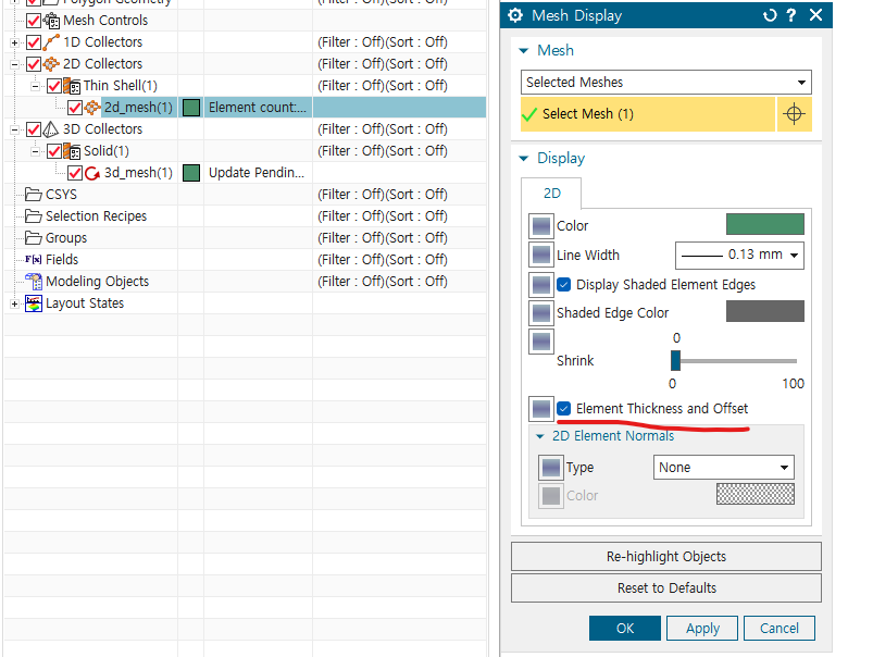
Cf) midsurface 2D mesh 입체로 보기
- 2d mesh -> edit display -> Element Thickness and Offset true
4. solution
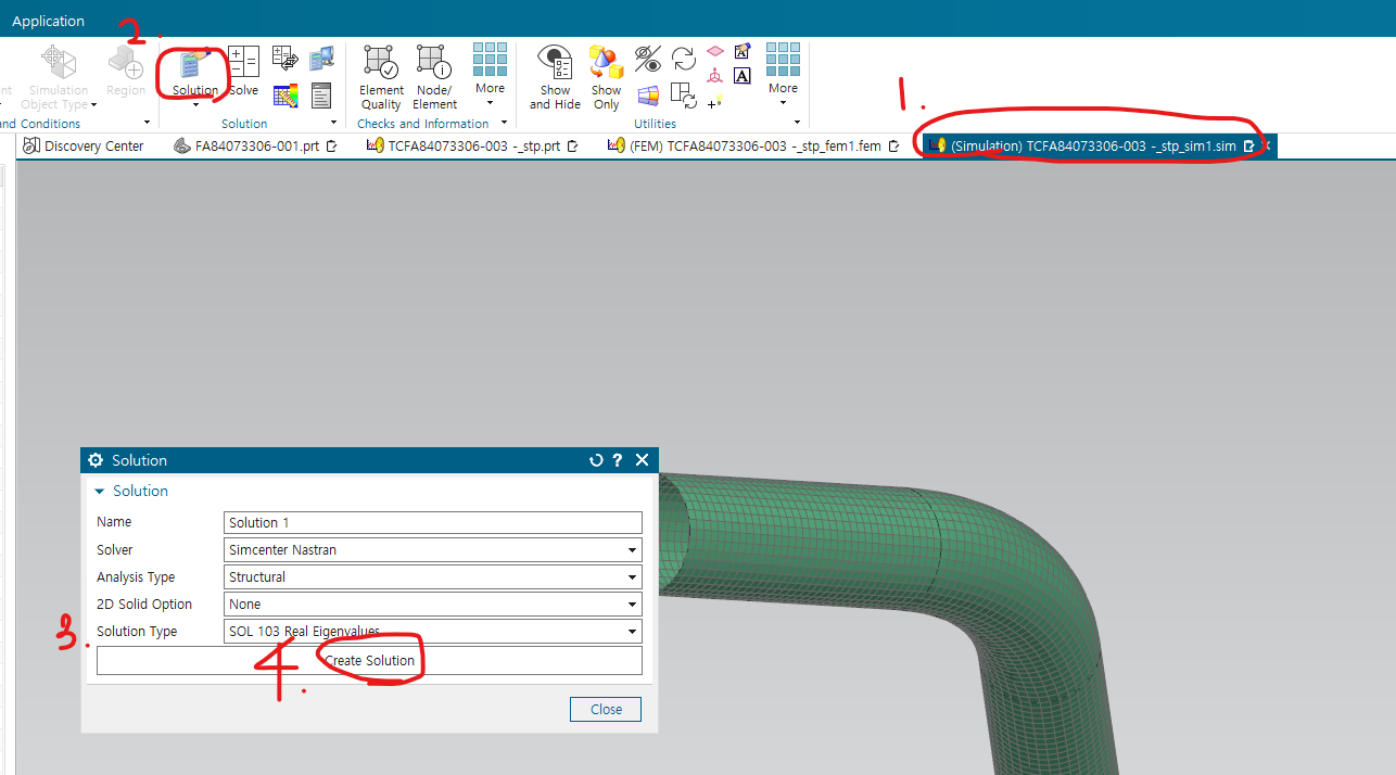
1) modal analysis
1. simulation으로 이동 -> 2. soultion -> 3. solution type을 sol 103 real eigenvalues로 선택 -> 4. create solution 클릭
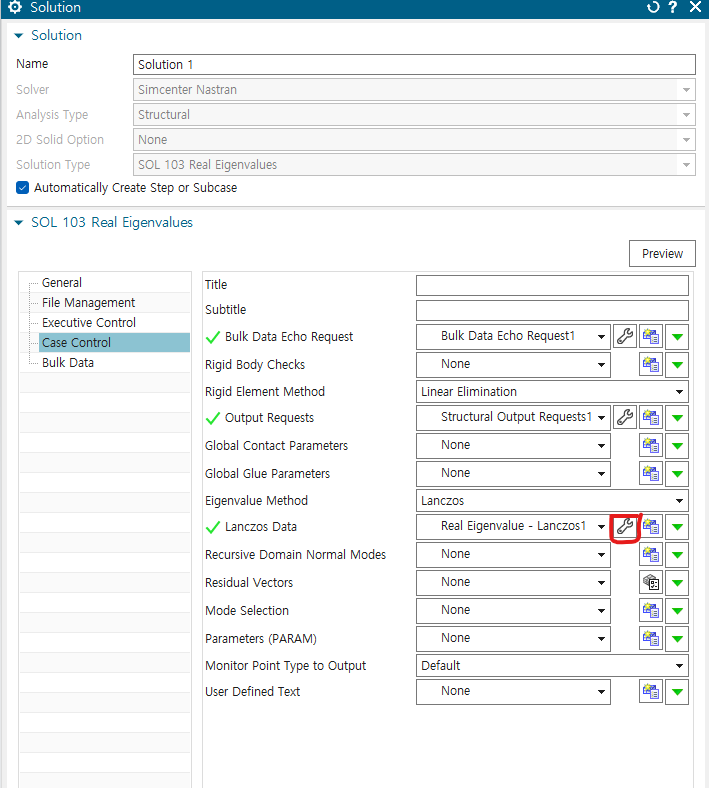
추출할 mode 개수 선택 - Lanczos data의 도구 모양 선택하여 설정
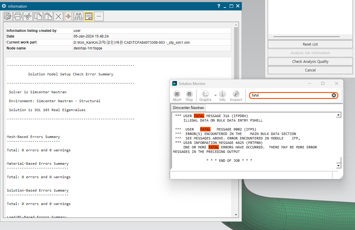
solve 누르고 information에 error가 있는지, solution monitor에 fatal이 있는지 확인
1-1) 결과 확인
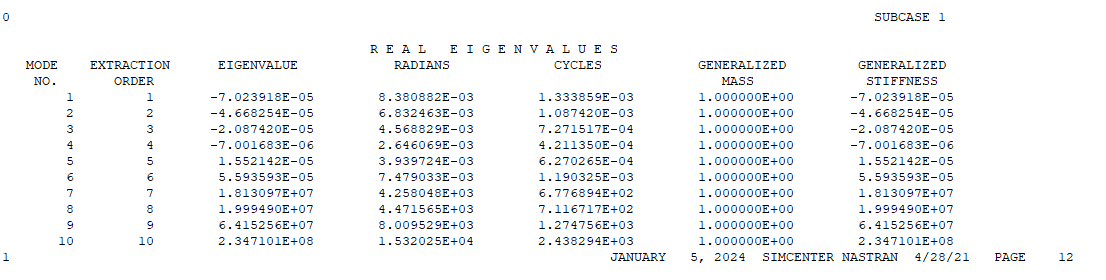
이렇게 solve를 진행하면 .f06이라는 확장자로 데이터가 저장되는데 여기서 각 mode의 eigen-value를 확인할 수 있다.
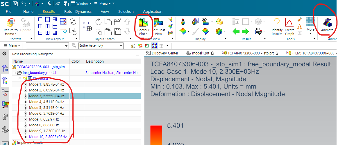
만약에, free - boundary condition으로 실험을 진행하게 된다면, 1-6번은 rigid motion에 대한 데이터고 7번 부터 진동에 대한 고유값을 의미한다. 또한 eigenvalue는 w의 제곱으로 진동수 Hz의 단위로 나타낼 때에는 고유값을 제곱근 한뒤 2pi로 나눌 것 !!
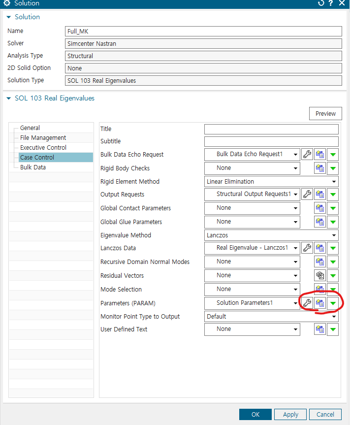
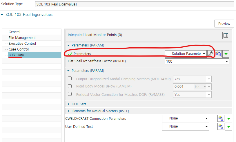
1-2) full mass stiffness matrix 필요한 경우
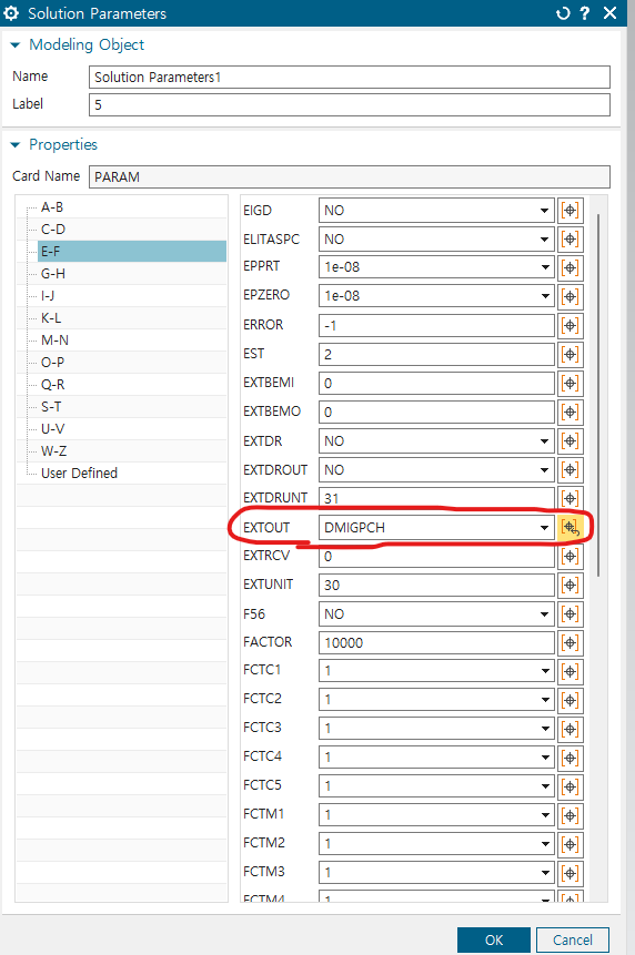
solution에서 103 Real eigenvalues -> param의 도구 -> extout option을 DMIGPCH로 바꾸기(E-F로 되어있는 것 중에서 찾아서 하기)
그러면 결과가 .pch 파일로 나옴 이를 matlab 코드로 mass와 stiffness matrix 얻기
2) 103 superelement를 이용하여 rom으로 mass, stiffness matrix 얻기
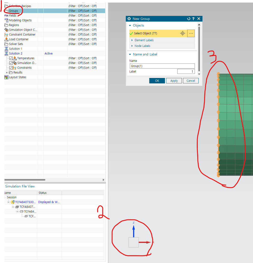
2-1) boundary condition 지정하기
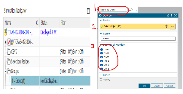
1. groups 더블클릭 -> 2. 정육면체 모양의 툴로 방향 조절하면 수월함 -> 3. 드래그해서 원하는 boundary condition 지정
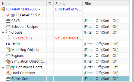
solver set우클릭 -> new -> Dof set
1. Nodes by group -> 2. select object는 왼쪽 창에서 원하는 그룹 선택 -> Dof 모두 선택 (x,y,z 회전 병진)을 모두 고정
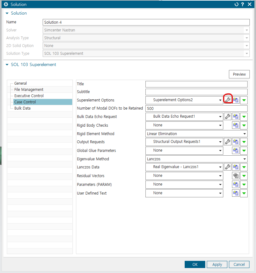
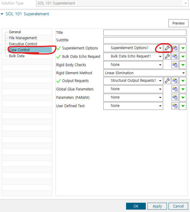
2-2) 103 superelement solution
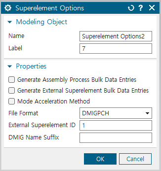
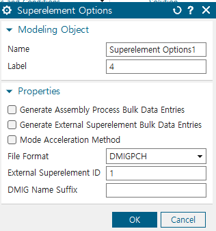
superelement Options의 도구에 들어가기
file format을 DMIGPCH로 지정, external superelement ID는 1로
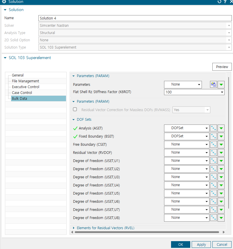
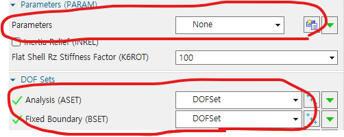
bulk data에 들어가서 Dof sets의 analysis와 Fixed boundary에 이전에 지정한 Dof set을 넣기
solve 진행하고, .pch파일을 matlab 코드를 이용해 reduced matrix 얻음
5. Modal analysis 결과 animation으로 확인하기
Results->Structural 더블 클릭
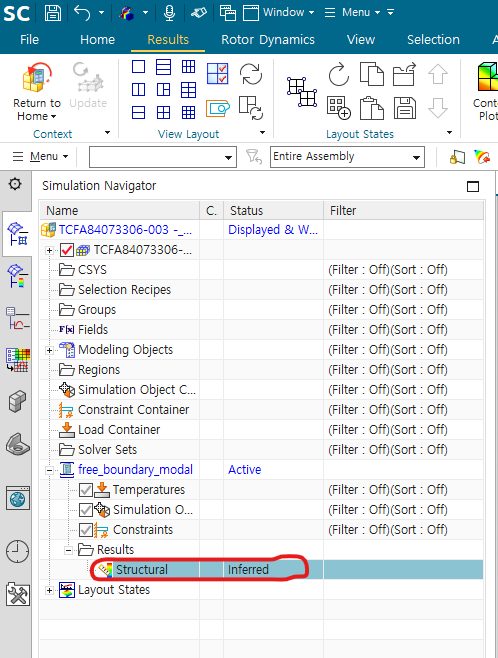
원하는 mode 선택 -> Contour plot -> animate
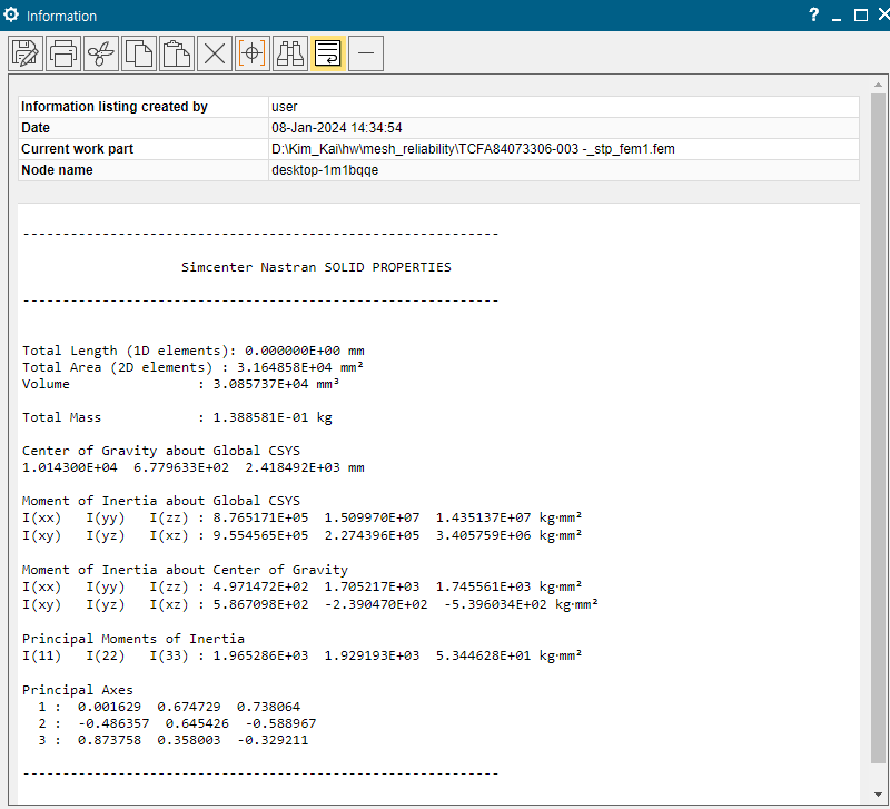
6. CF) 질량 체크
fem -> 돋보기에 solid properties check 클릭-> units를 kg-mm로 설정
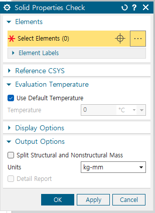
total mass 정보 확인 가능
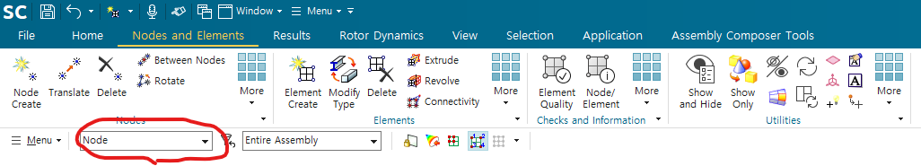
7. Point Mass 입력
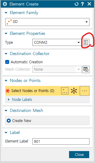
Tool bar의 Nodes and Elements의 Element create 선택
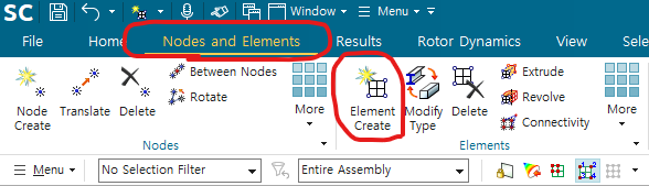
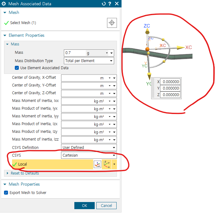
Element Family는 OD, type은 CONM2로 그리고, Type 옆에 체크 동그라미 표시에 들어가 질량 입력
특이 케이스 - 고정부 방향이 틀어져 있는 경우
- Csys - Cartesian에서 Local 좌표계 설정
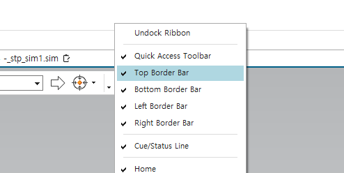
우클릭해서 Top Border Bar 선택하기
그리고 노드 선택 버튼을 눌러, 노드에 질량을 부과할 수 있도록 함.
Point mass CONM1 CONM2차이
CONM2 : Concentrated mass and inertia terms at a grid point via a CONM2 Bulk Data entry. The provisions
of the CONM2 entry are the mass, the offset of the center of mass from the grid point, and the
moments and products of inertia about the center of mass. As an option, the center of mass may
be measured from the origin of the basic coordinate system rather than as an offset from the
grid point.
CONM1 : A full 6 × 6 symmetric matrix of mass coefficients at a grid point via the CONM1 Bulk Data entry.
-
즉 CONM2 는 mx my mz Ixx, Iyy, Izz, Ixy, Ixz, Izy 와 해당 point로부터 질량 중심의 거리만을 입력함.
-
그러나 CONM1의 경우에는 6 by 6 mass matrix의 coupling 성분들을 모두 입력 가능
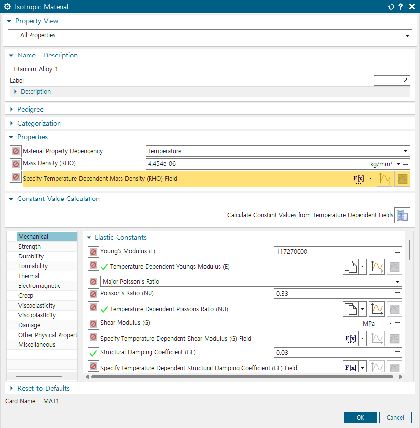
8. damping coefficient 입력
material에서 원하는 물성치 우클릭 -> copy
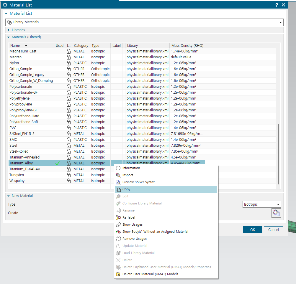
3% - 0.03을 structural damping coefficient에 입력
9. Craig_bampton위한 mode extract - 103 superelement
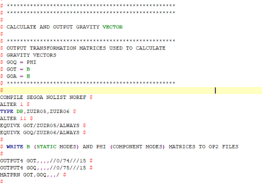
CB Matrix를 통해 여러가지 구조해석을 진행하기 위해서는 CB Method Transformation Matrix를 생성해야 한다. Simcenter에서는 바로 Transformation Matrix를 생성해 주지 않아, Nastran의 DMAP 언어를 사용해 해석 도중 생성되는 Transformation matrix의 성분(ψ,ϕ)을 파일로 생성하였다.
Transformation matrix를 생성하는 DMAP 코드는 다음과 같다. Simcenter해석에서 PSI(ψ)는 GOT 로, PHI(ϕ)는 GOQ로 나타낸다. 따라서 해석 도중 해당 성분을 생성해내는 코드를 이용한다.
solution -> filemanagement -> user defined text
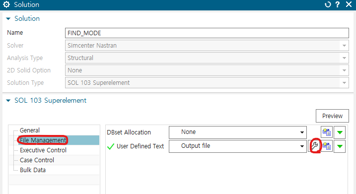
name : Output file, text to insert at start of section의 keyin text는 아래의 코드 입력
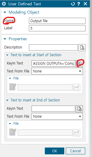
ASSIGN OUTPUT4='Comp_b.ext' ,
UNIT=74 STATUS=UNKNOWN FORM=FORMATTED
$
ASSIGN OUTPUT4='Comp_e.ext' ,
UNIT=75 STATUS=UNKNOWN FORM=FORMATTED
추가 설명 : DMAP 해석 결과를 저장하기 위한 파일을 생성하기 위한 과정이다. File Management card에서 User Defined Text를 이용한다. 위의 DMAP Code에서 PSI는 74번, PHI는 75번으로 설정하였으므로, 해당 코드를 UNIT으로 지정한다.
dmap 코드 입력
Executive Control의 User Defined Text에 들어감
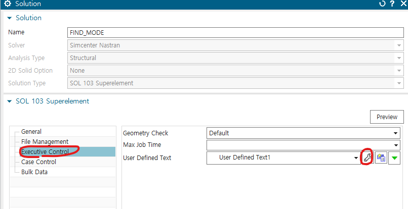
text to insert at end of section의 keyin text는 아래의 코드 입력
include 'fedem_dmap_i04.dat'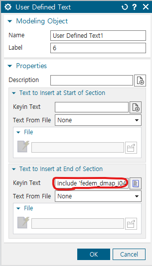
결과 파일 comp_e.ext 에는 PHI가 comp_b.ext에는 Psi가 저장됨
10. couple system
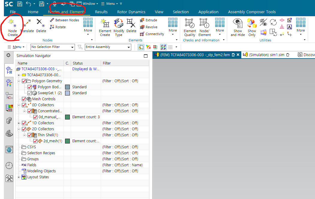
point(node) 생성
-fem -> node and elements -> Node create
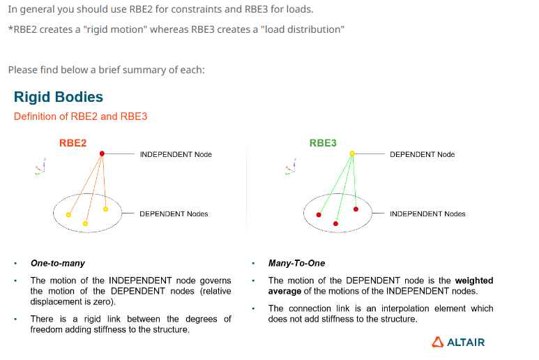
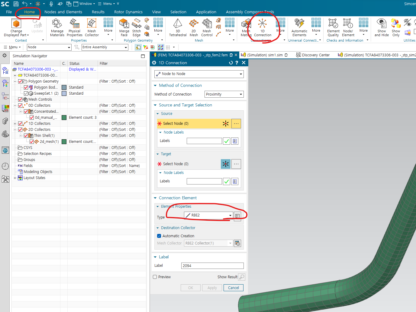
connection 생성
-home -> 1D connection에서 RBE2 설정 , target, source 선택
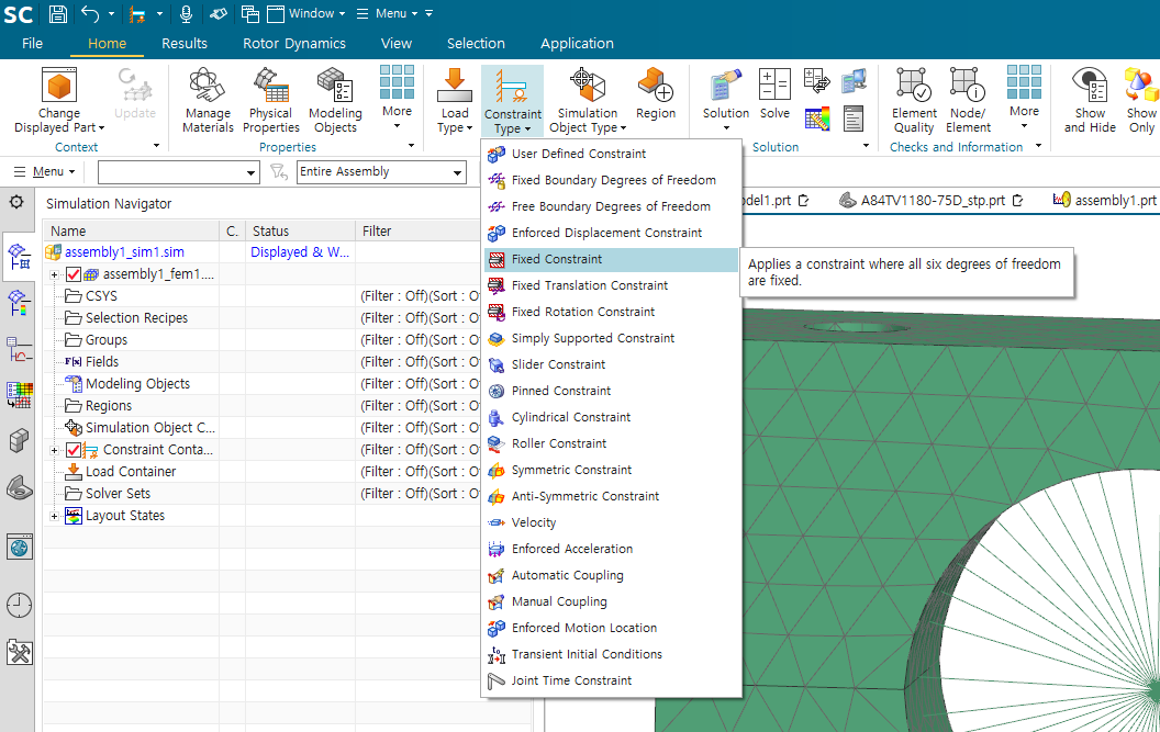
fixed constraint 적용
reduced matrix 설정
--> solver set을 중심 노드만 선택(아니면, 중복으로 인해 오류 발생)
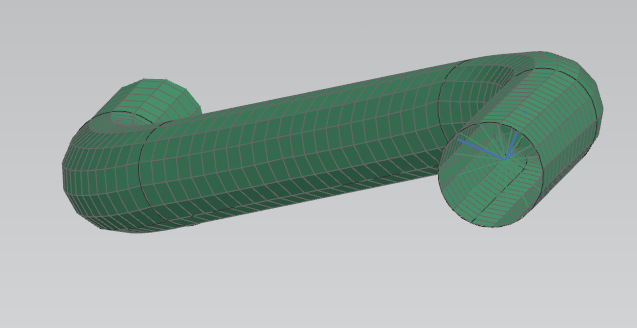
11. static analysis
assembly 할 때 유의할 점 -> creo에서 assembly 후에 stp로 저장하기
sol101-global 사용시
constraint와 load를 solution 생성 후, solution 내부에서 만들어야 함
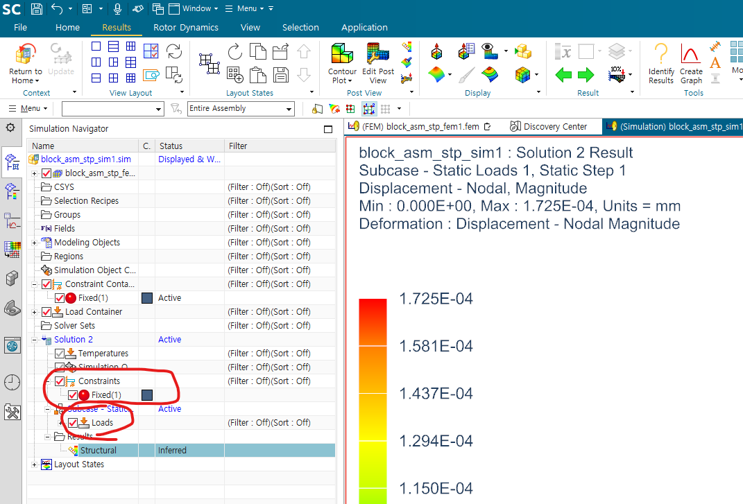
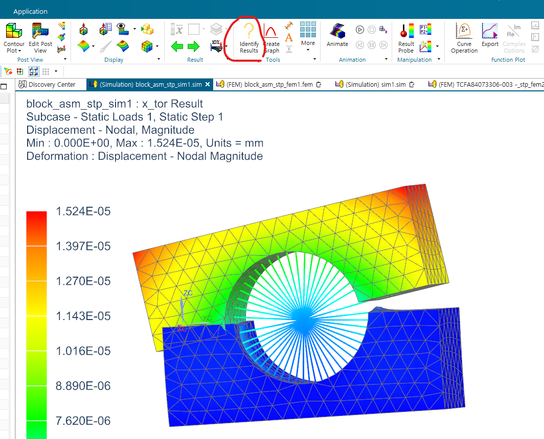
원하는 노드의 static deformation 확인 -> Results의 identify Results 기능 이용
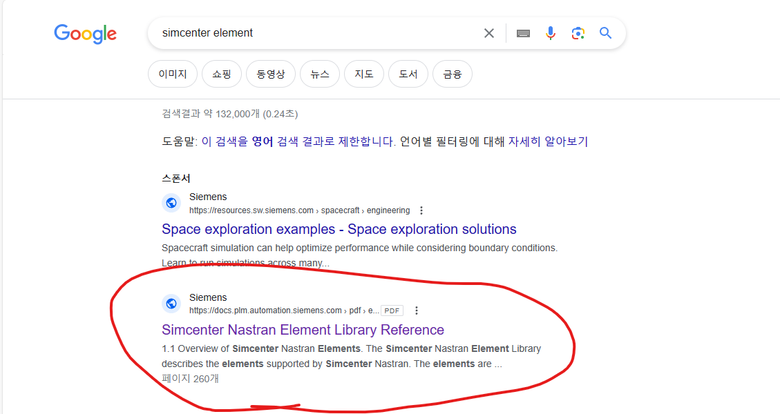
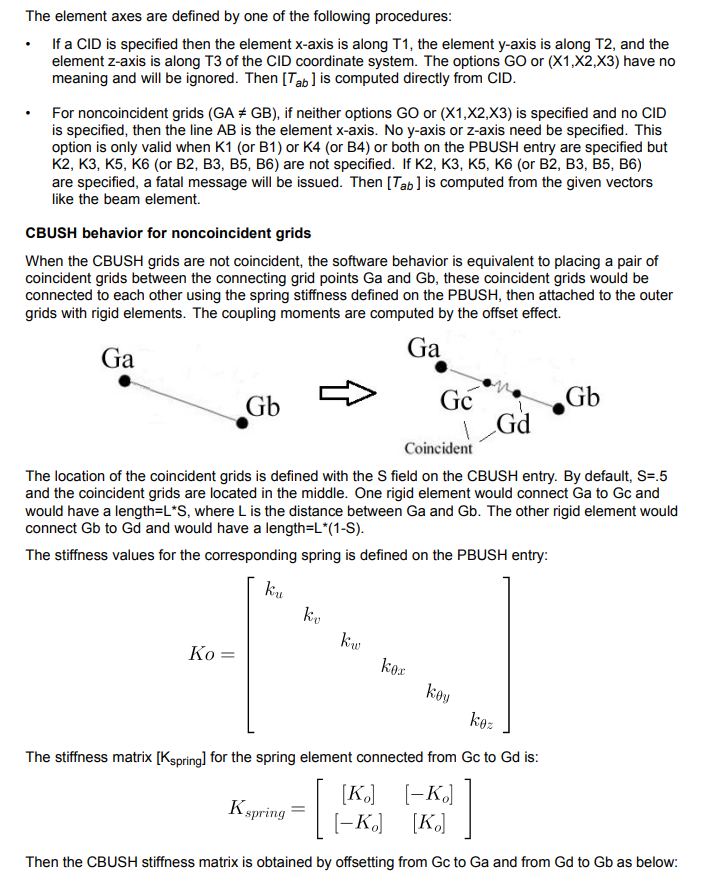
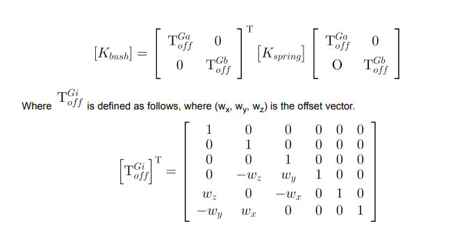
12. CBUSH로 최적화 실행
google에 simcenter element 검색 -> 아래의 pdf 확인 -> cbush 검색
cbush 생성 : 1D connection에서 잇고자 하는 두개의 노드 선택
source, target node 정하고, cbush 옵션으로 진행
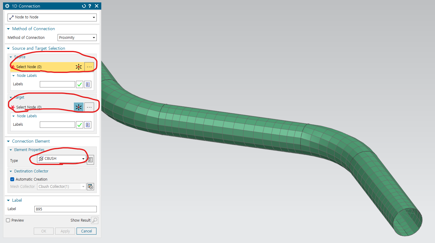
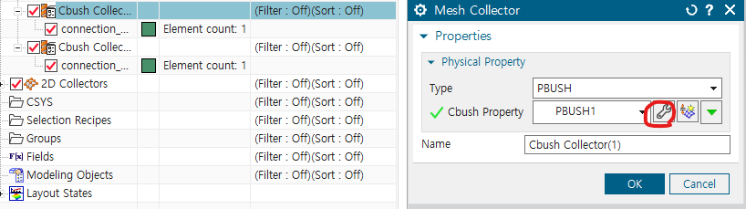
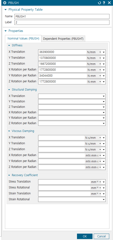
cbush 설정: cbush 도구 -> push1 옆의 도구 모양 들어가서, 강성, 감쇠 입력
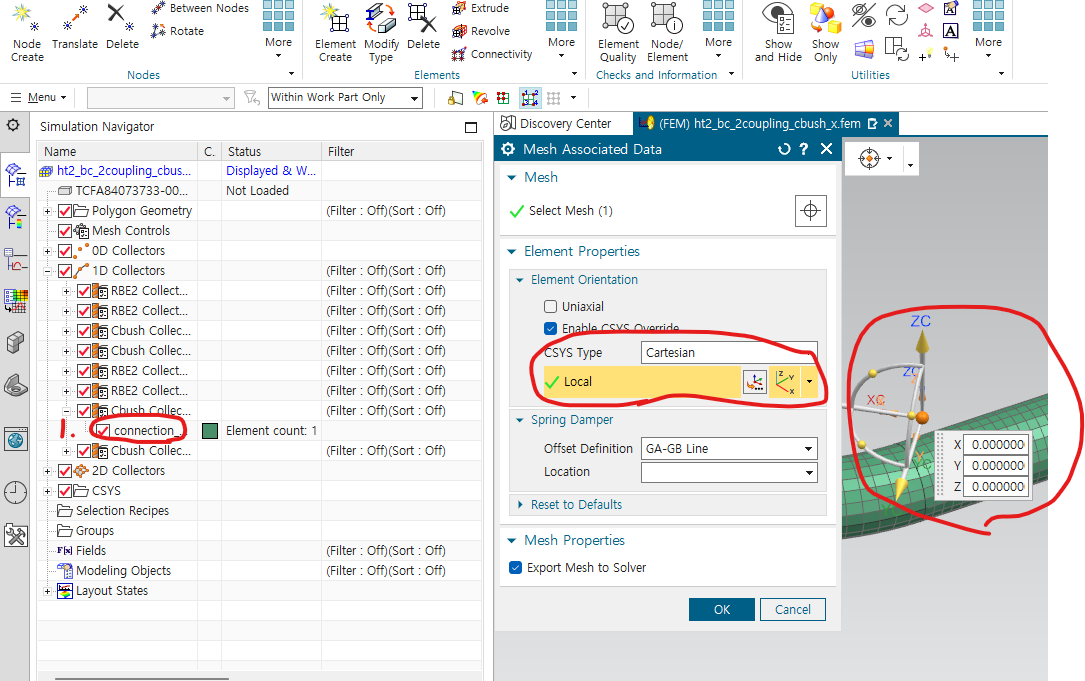
cbush 방향 입력-> cbush 아래의 connection -> edit mesh associated Data -> enable CSYS Override -> Absolute
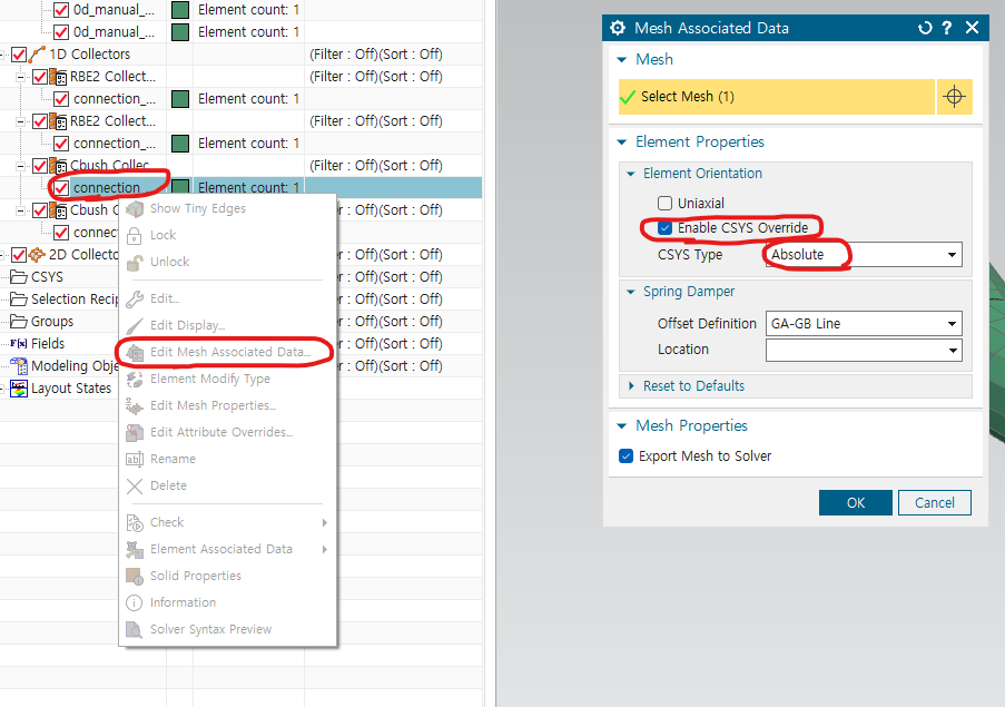
** 단 입구가 global 좌표에 대해 회전한 경우에는 다르게 해야 함.
enable CSYS Override -> cartesian -> local 좌표계 생성
modal 해석
->cbush로 연결한 반대편을 fixed constraint로 설정하기!!
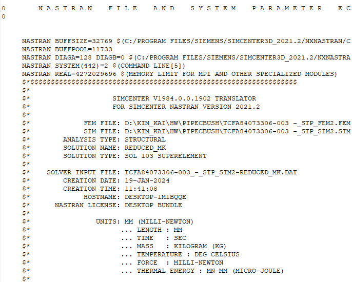
simcenter matrix 단위 조심
- 이거 보면은 단위가 mm, mN임 조심
matlab에서 cbush 포함한 k matrix 생성 아래 내용 참조
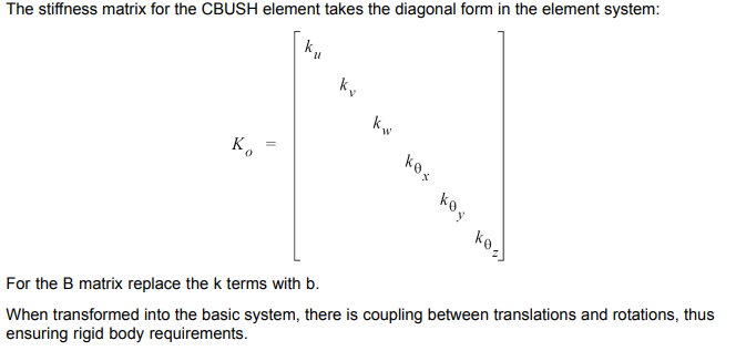
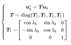
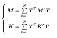
local coordinate로 cbush를 생성한 경우, matrix의 선형 변환을 이용해야 함.
- kx ky kz랑 krx kry krz 따로 적용시켜야 함
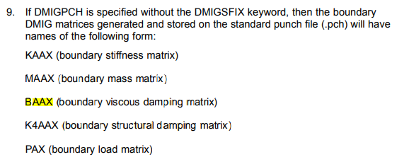
simcenter damping 종류
BAAX : viscous damping
K4AAX : Structural damping
13. Cbush로 damping 넣기 전과 후 비교하기
1) structural damping의 경우
1 재료 물성치를 통해, structural damping 넣고, cbush에도 structural damping coefficient 넣어서 superelement 103을 통해서 reduced된 m,c,k 뽑음
2 재료 물성치에만 structural damping 넣고, cbush에는 structural damping이 안들어간 reduced 된 m,c,k 뽑기
1에서 구한 c matrix에서 2에서 구한 c matrix를 빼서 어떤게 달라졌는가 볼것
2) Viscous damping의 경우 (좀 더 복잡)
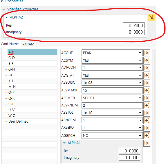
1 solution type 103 Real Eigenvalues의 case control -> param extout에서 dmigpch 설정, Bulk data -> params에 들어가, alpha2에 아무 값을 입력하고 Full m,c,k 뽑기
2 solution type에서 103 superelement로 reduced된 m,k와 psi,phi 뽑기
3 solution type에서 101 superelement로 cbush에 damping이 들어간 reduced된 m,c,k 뽑음 (101 superelement는 modal domain없음 주의)
4 1에서 Full m,c,k에 2에서 psi와 phi로 구한 Transformation matrix를 연산하여, reduced된 m,c,k 계산
4의 reduced된 c와 3의 reduced된 c를 비교
- 결론 : cbush에서 강성, 감쇠를 넣어도, psi,phi, psi_cb와 modal domain은 항상 동일함
contact condition

simulation object type에 들어가기
14. Harmonic analysis
-
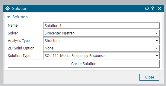
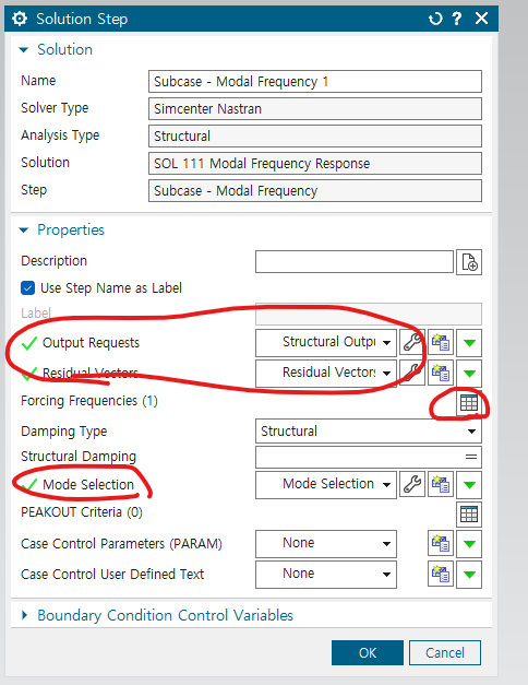
solution의 sol111 modal frequency response 이용
-
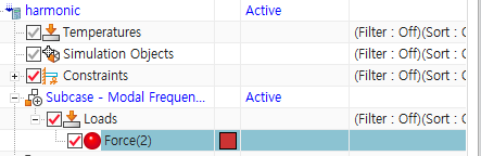
원하는 노드에 force 생성
-
solution edit -> force frequency 정의
이거 할때, output requests lancoz data도 활성화
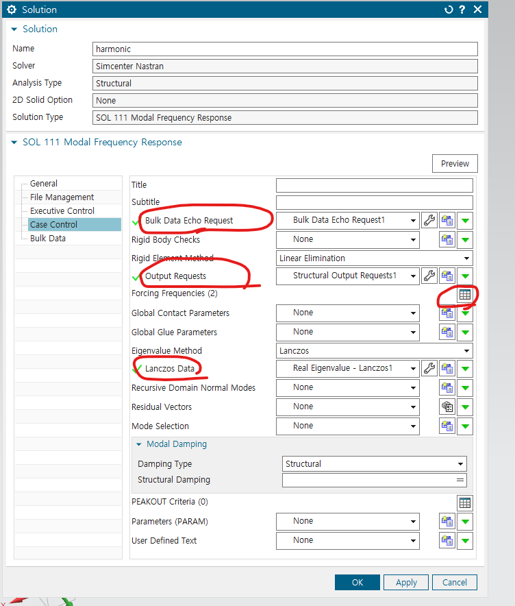
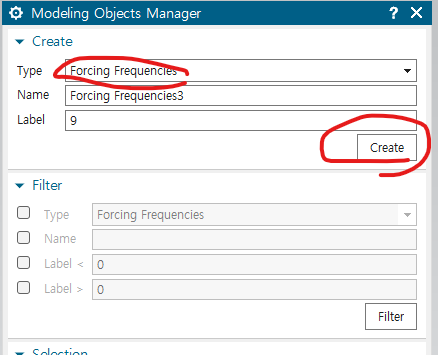
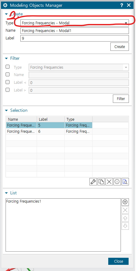
2가지 방법으로 frequency 생성 가능
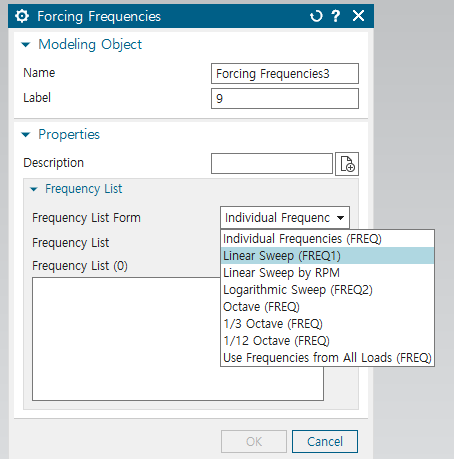
1. 일반적으로 frequency 생성
-
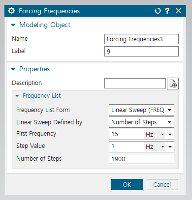
원하는 옵션 선택
-
시작 주파수, 주파수 간격, 간격 수 결정
-
원하는 forcing frequency 고르고 + 버튼 누르기
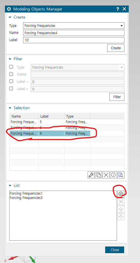
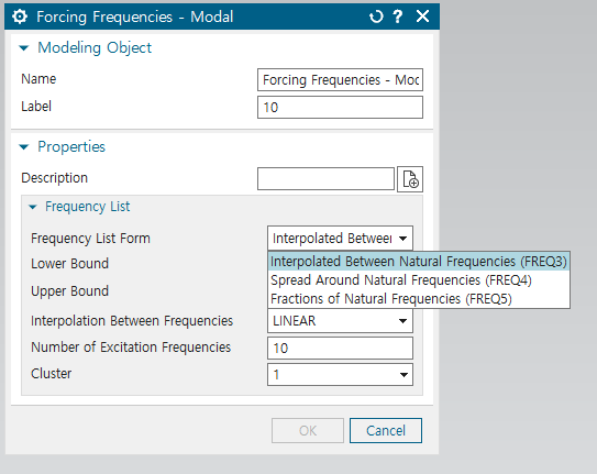
- 고유 진동수에 대한 상대적인 비율, 고유진동수 주변으로 frequency 생성
- 해당 옵션중 원하는거 선택 -> 이후에는 1번 방법과 동일
- 그 후 subscase modal frequency 에서도 forcing frequency 동일하게 지정
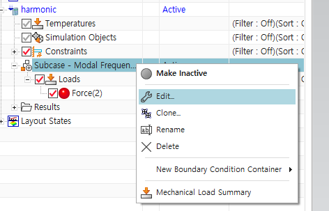
- 여기서 output request, residual vector, mode selection도 활성화
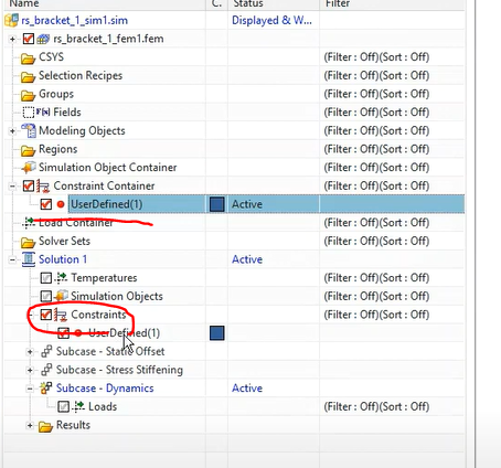
15. Response dynamics 생성 방법
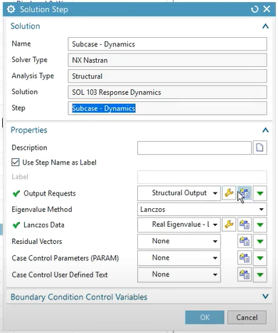
1) solution 생성 - sol 103 response dynamics
- subscase - dynamic edit
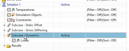
- output request 설정
-
enable acceleration request
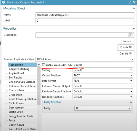
-
constraint 적용
-
선택사항 : constraint - enforced motion location
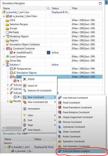
이런식으로 여러 노드에 특정 방향으로 enforced motion 구속 조건 적용 가능
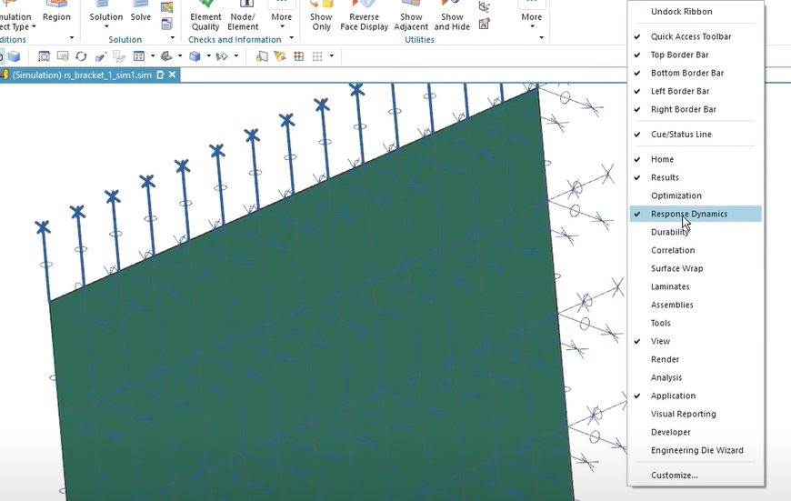
-
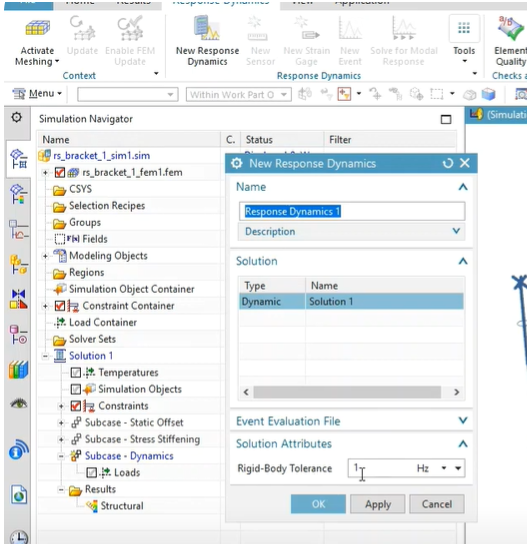
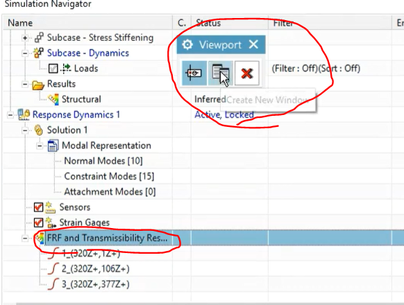
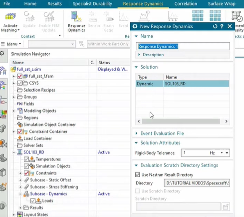
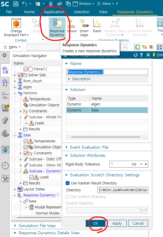
solve 후 tool바에서 우클릭 -> Response Dynamics 창 생성
-
response dynamics의 New response dynamics 생성
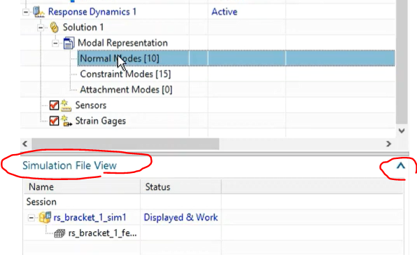
- 새로 생성된 response dynamics 1 의 normal mode를 simulation file view를 확장시키면 확인 가능함
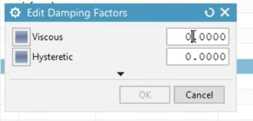
- damping 요소도 첨가
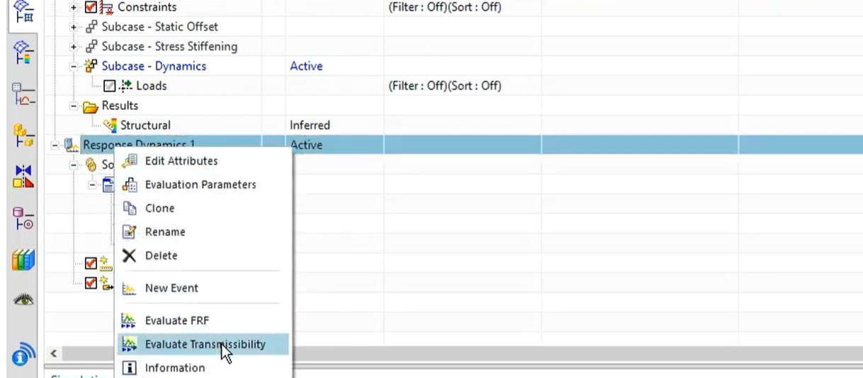
- evaluate transmissibility
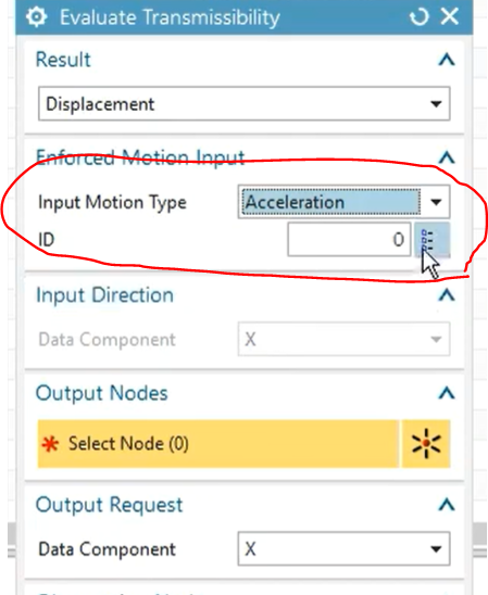
- input motion type - acceleration
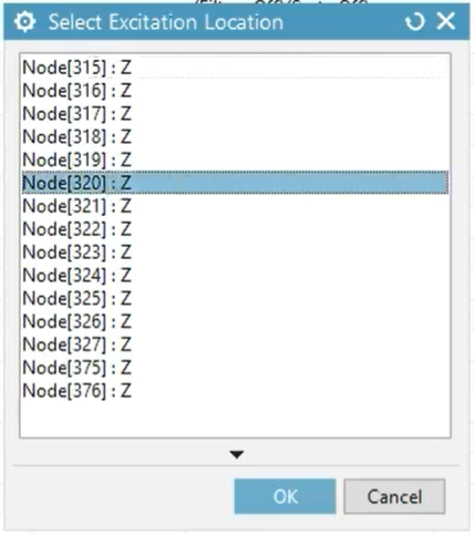
- 원하는 input data 노드 선택
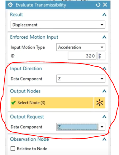
- input direction, output direction, output node 선택
- transmissibility 그래프 그리기
16. Base excitation
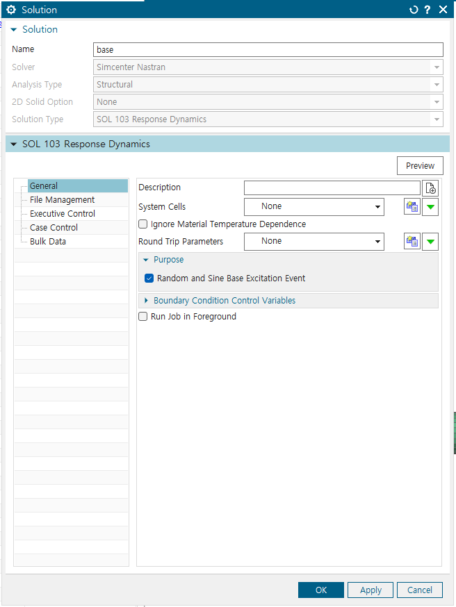
1) solution 생성과정
solution type SOL 103 Response Dynamics
- purpose에 Random and Sine Base Excitation Event
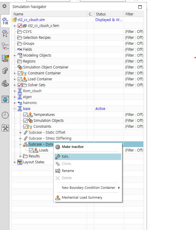
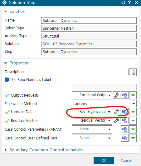
2) Subcase option 지정
Subcase - Dynamics - Edit
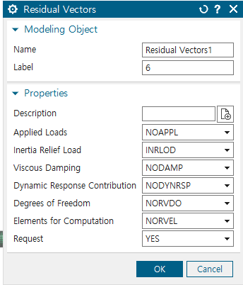
residual vector 지정
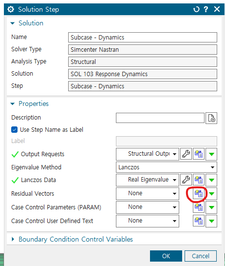
이 세팅으로 (random solution의 정확도 향상을 위해)
- inertia relief load 말고는 다 비활성화
Lancoz Data에 들어가서 추출할 모드 주파수 범위, 개수 지정
3) constraint 지정
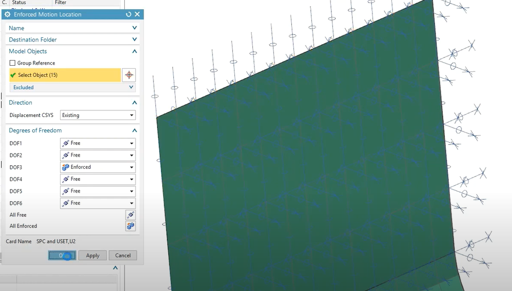
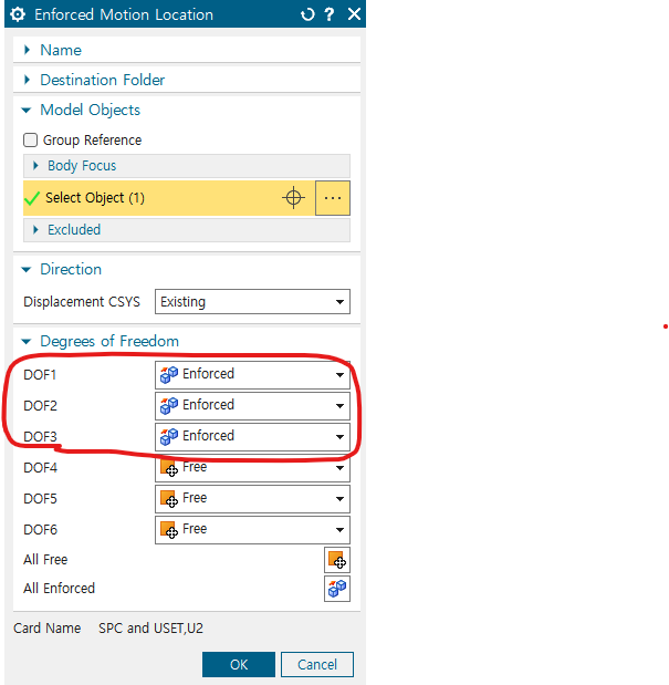
3-1) constraint type enforced motion location에서 원하는 노드 선택, Transitional 을 담당하는 DOF1~3 Enforced, 나머지 torsional 부분은 free로
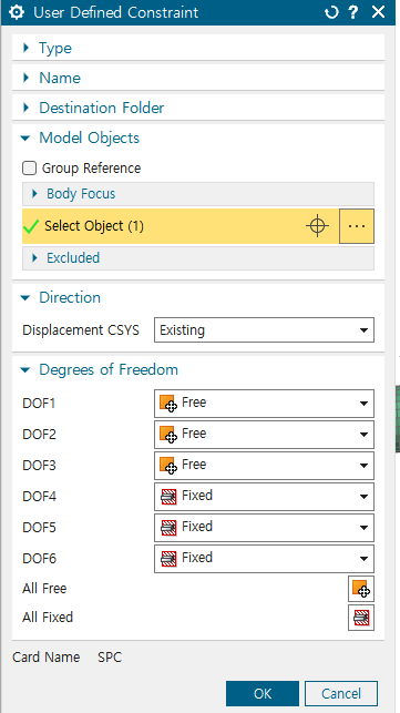
3-2) fixed constraint 지정 -> user defined constraint에서 원하는 노드 선택 -> DOF 4~6을 fixed로 나머지는 free
- 여기서 주의 할 점 : endforced motion location 노드는 1개만 선택 (Base excitation의 경우)
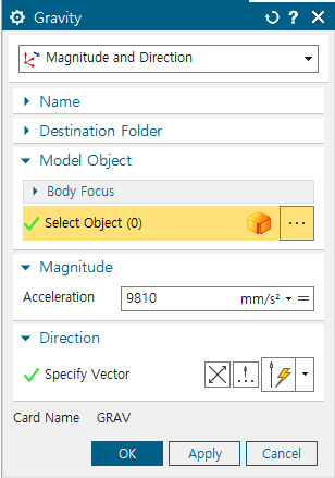
- 중력 넣을 수도 있음
4) solve 이후 Option 지정
4-1) Response Dynamics 창에서 new Response Dynamics 선택
4-2) 원하는 해석 유형 결정 (Base에 PSD 적용 후 원하는 노드의 가속도 측정 혹은 Base와 원하는 노드 사이의 Transmissibility 계산)
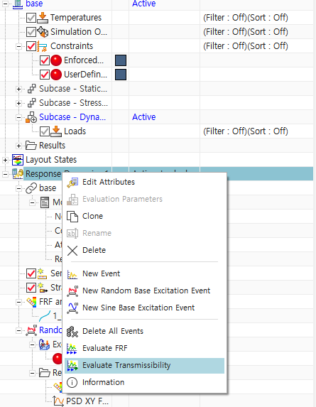
- Transmissibility 계산하는 경우
- Response Dynamics 우클릭 -> Evaluate Transmissibility
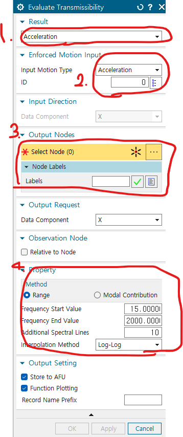
1) result를 acceleration으로
2) input motion type을 acceleration으로 선택, ID는 위에서 정한 base의 노드 입력(Enforced motion location이랑 fixed constraint를 가한 노드)
3) output node 선택
4) 주파수 범위 입력 Additional Spectral lines를 증가시켜, frequency를 더 잘게 쪼개어 해석 가능
- 좌표 맞추기
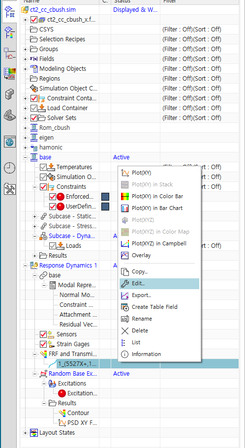
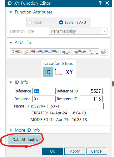
생성된 FRF and Transmissibility 우클릭 -> Edit
data Attribute 선택
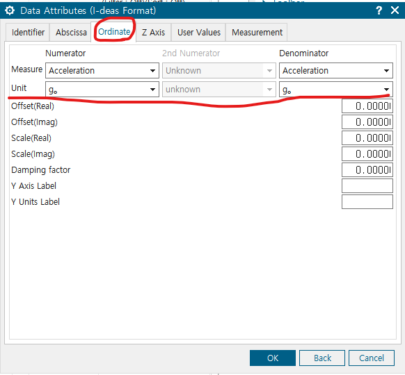
ordinate에서 분자 분모 단위 선택
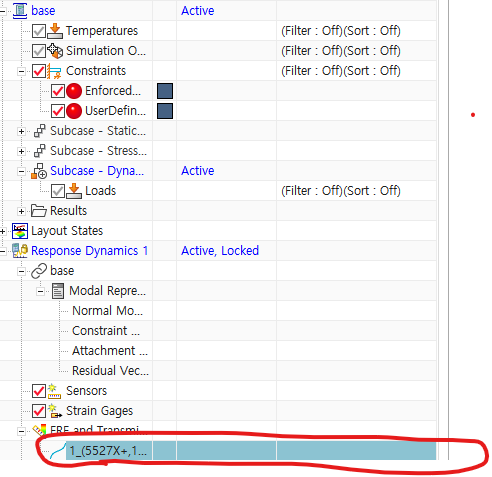
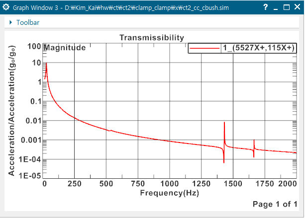
그리고 Response Dynamics 하부의 FRF and Transmissibility에서 결과 확인 가능- 해당 지점에 우클릭 -> Plot(xy)
- 그리고 create new window 옵션 선택하면 아래와 같은 Transmissibility 나옴
- Export result
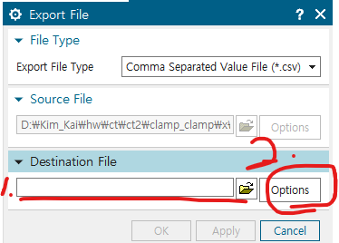
동일한 지점 우클릭 -> Export
1) 저장 경로 지정
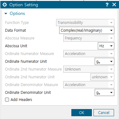
2) output file option 선택
option은 분자 분모 모두 G이므로, 단위 바꿀 것
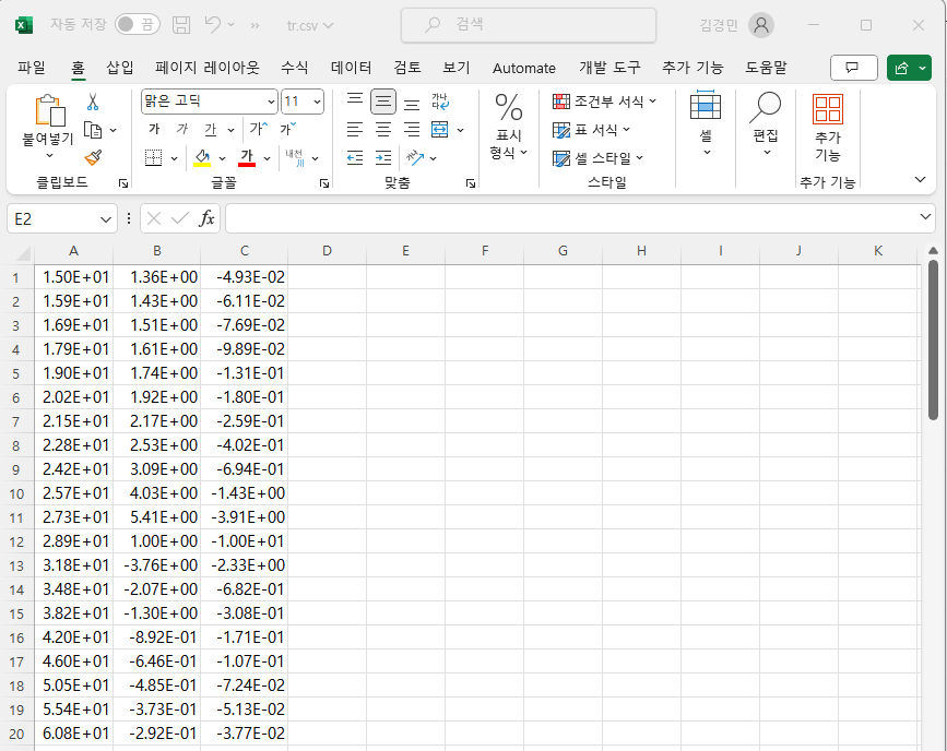
Csv 파일
1열 : 주파수, 2열 : y 값의 Real part, 3열 Imaginary part
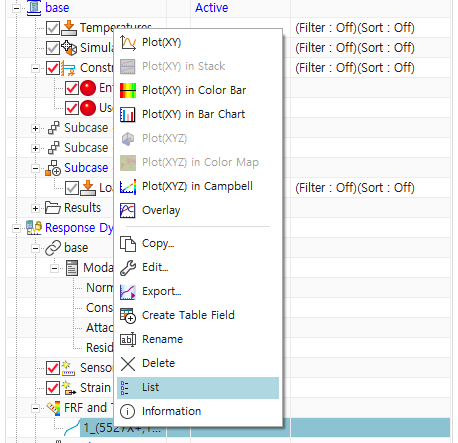
- 혹은 우클릭 -> list에 들어가서 html 파일로 저장 가능
- PSD를 이용한 Random Base Excitaion
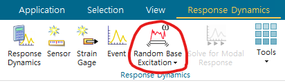
- response Dynamics 생성 후 -> Random Base Excitation 생성
수정 사항들
1) 옵션 세부 선택
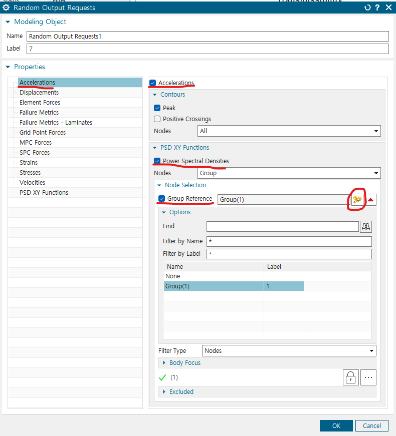
- 가속도 결과를 볼 것이므로 Acceleration에 들어가서, Acceleration, Power Spectral Densities 체크
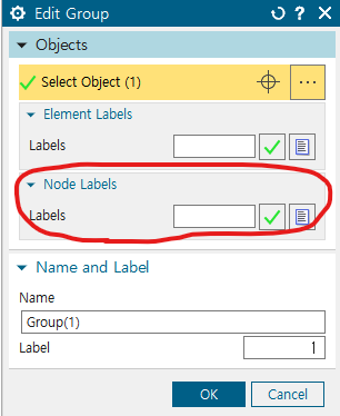
- node selelction은 Group reference 체크하고, 우측의 동그라미 버튼 (Edit Group) 눌러서 그룹 설정
PSD 결과를 확인하고 싶은 node 선택 혹은 Element 선택 후 OK 버튼 누르기
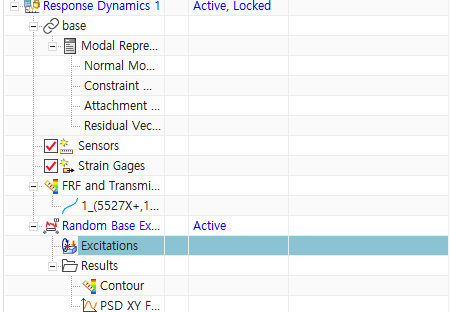
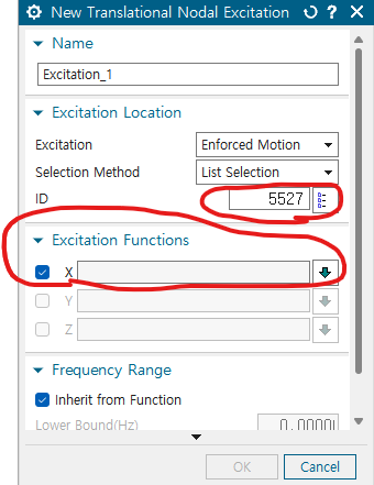
Response Dynamics -> Random Base Exictation -> Excitations에서 우클릭- new ecitation -> Transitional Nodal 생성
- 먼저 Excitaiton Location의 ID에는 이전에 Enforced motion location constraint를 지정한 노드의 번호가 들어감
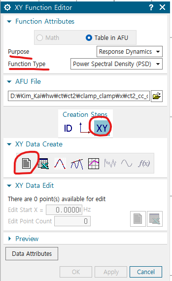
- 그리고 Excitation Functions에서 PSD 프로파일 입력하기
Function manager -> New 선택
- Purpose : Response Dynamics (Default)
- Function Type : PSD (Default)
- Creation Steps -> XY (x,y 데이터를 가지고 있었기 때문에 이거 쓰는게 편했음)
- XY Data Create -> txt file (이거 쓰는게 제일 간단한거 같음)
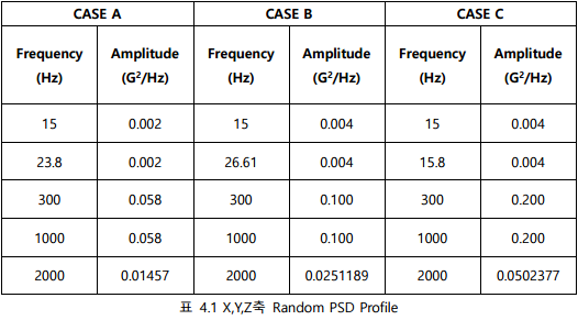
- 기계 연구원에서 받은 PSD Profile (참조)
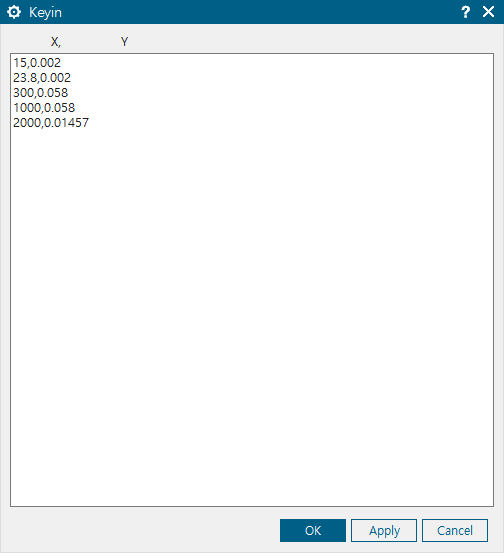
이런식으로 XY 좌표를 , 로 구분해서 입력하고 OK 버튼 누르기 (전부 다 OK 버튼 누를 것)
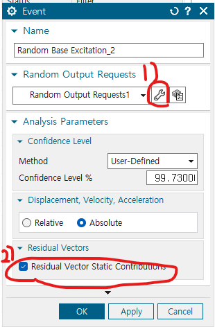
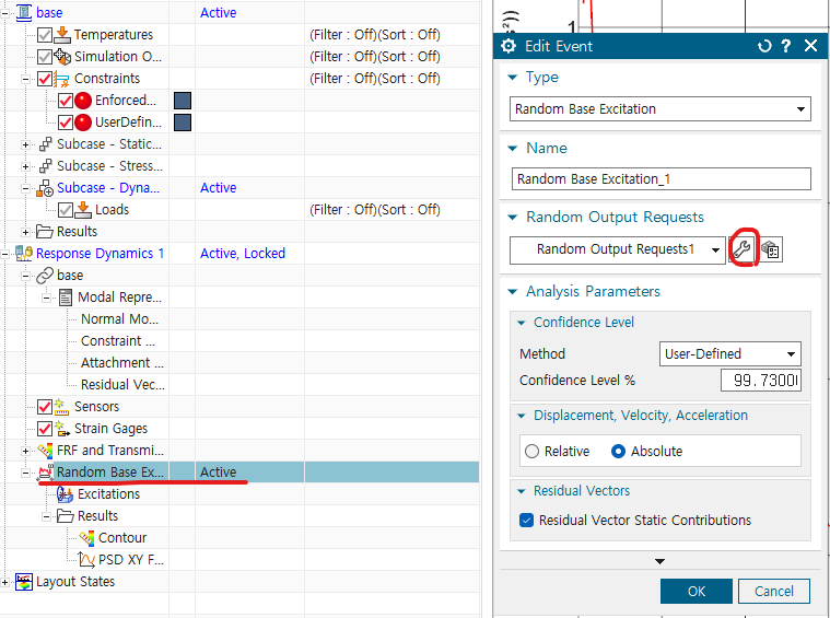
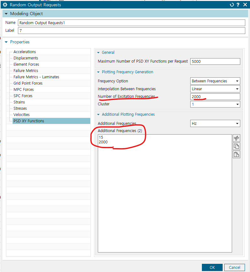
- 그리고 Random Base excitation 우클릭 -> Edit Attributes -> Random Output request 설정 들어가기
- PSD XY Functions의 Additional Frequency 입력 (PSD 지정했던 주파수 범위인 15~2000 Hz), Number of Excitation frequency 증가시키기, 해당 값이 커야, 그래프에서 Frequency 간격이 줄어드는 효과 발생
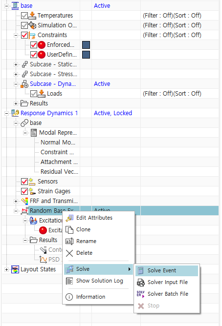
- Random Base excitation solve -> solve Event
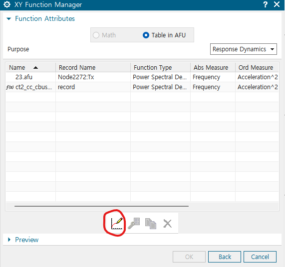
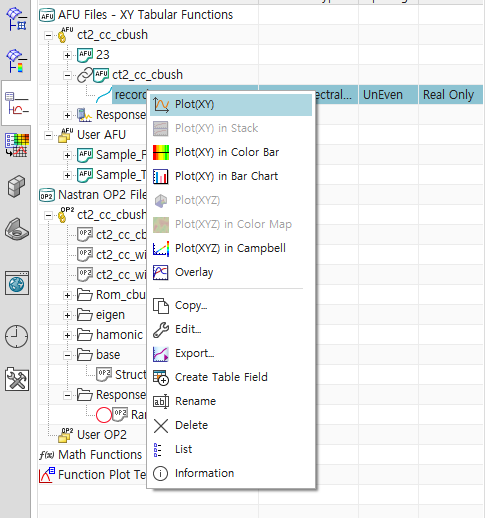
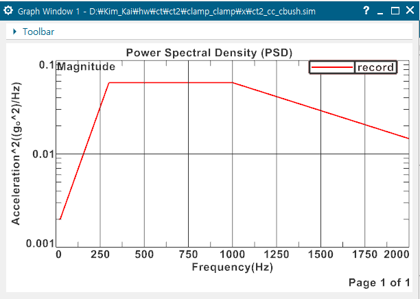
- 지정한 PSD Profile 확인하기 : XY Function Navigator의 ct2_cc_cbush(simulation 파일명) 하부의 record 우클릭 -> Plot(XY) -> Create New window
- 위에서 지정한 PSD profile (X축 Frequency, Y축 G^2/Hz)
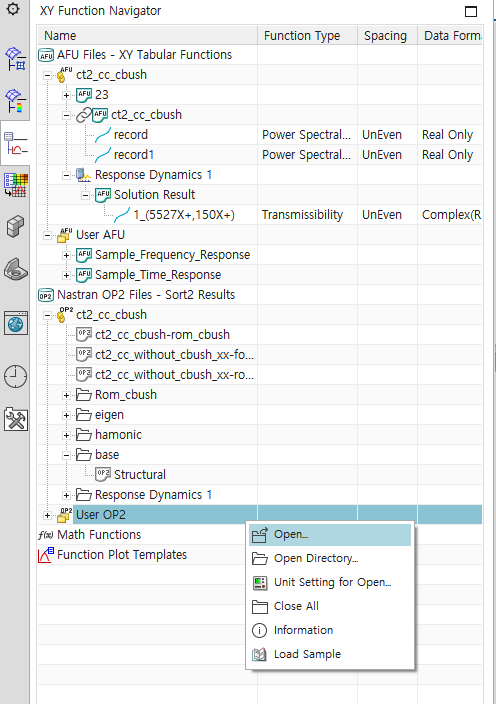
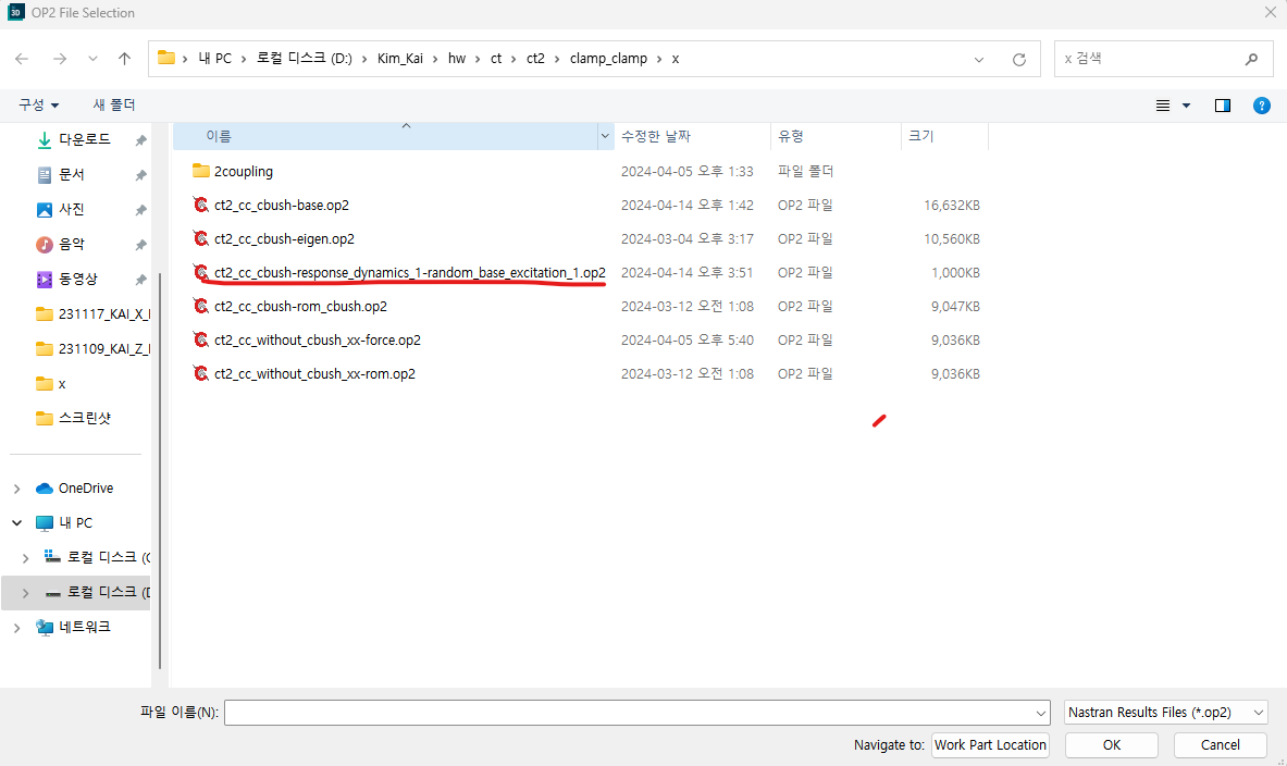
- user OP2 -> open
- Random base excitation OP2 file load
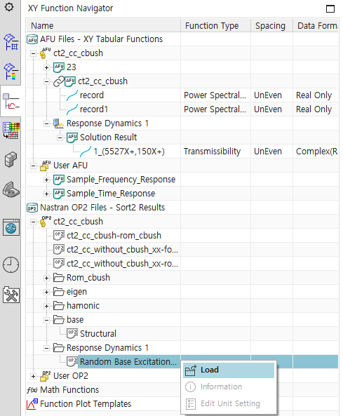
- 마지막으로 Response Dynamics 하의 Random Base Excitation Load하기
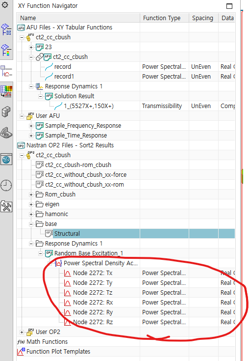
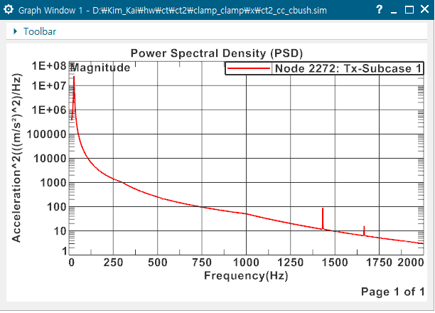
- 그러면 원하는 방향의 Random 가진 결과 (output PSD) 확인 가능
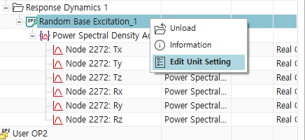
- 원하는 단위 설정
- 결과 그래프
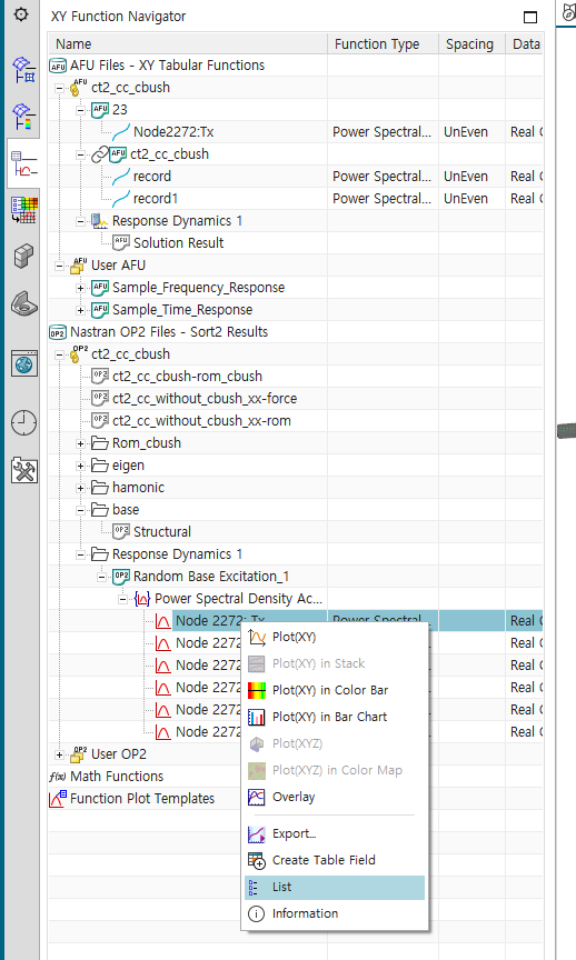
- 우클릭 -> list에 들어가서 txt 파일로 저장하기
x 값 주파수, y 값 amplitude
- Transmissibilty simulation 검증 과정
multi-dof transmissibility
1) coupling node와 센서 위치에 boundary node를 생성하여, Rom 추출
2) Couling node에 힘을 가하여, Transmissibilty 계산 -> 아래 식 참조
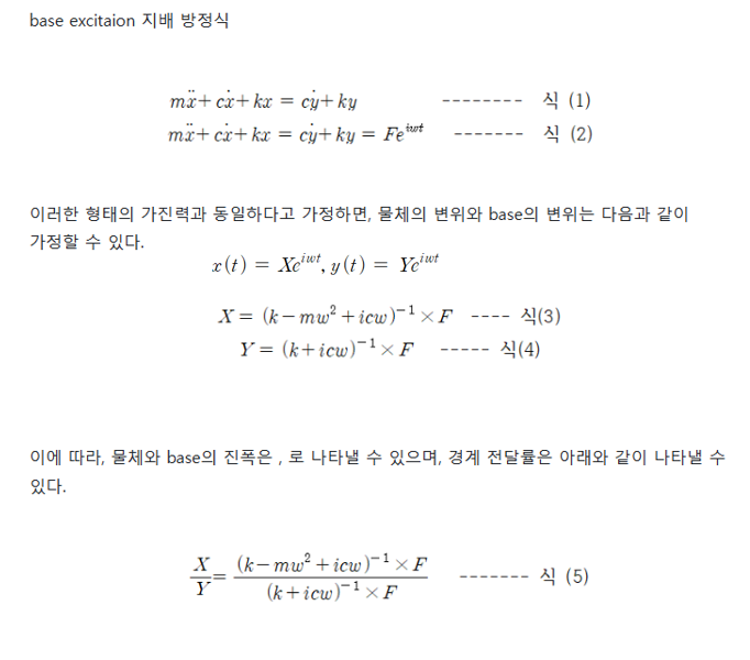
이때, 힘 F는 물체의 고정부에 가해지며, x 방향 힘인 경우, 해당 노드의 6 DOF 중 x transitional 성분에만 힘이 가해지는 것으로 하여 계산할 수 있다.
이는 structural damping 에서만 가능 -> Y는 base 진폭이므로 상수, structural damping에서, 감쇠는 주파수와 무관 (진폭에 비례하는 감쇠력)하므로 F는 모든 주파수에 대해서 일정한 열행렬이 됨.
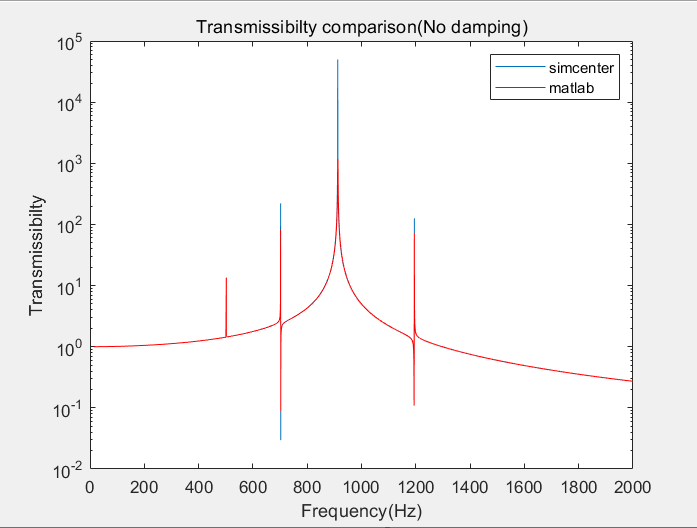
- simcenter와 matlab 비교 그래프
damping 없는 경우 (최대 상대 오차 700%, 평균 1.5%) -> damping 없으면 공진 주파수에서 발산하는 성질 때문에 공진점에서 높은 오차 발생
- structural damping이 20%인 경우
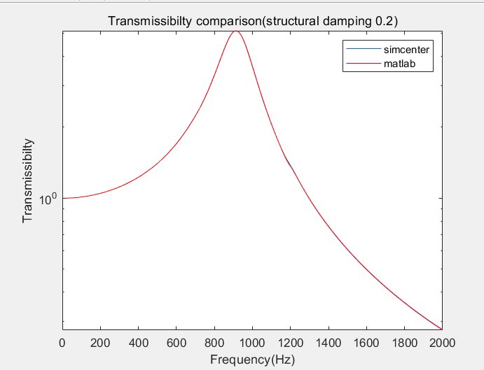
상대 오차 최대 0.24%
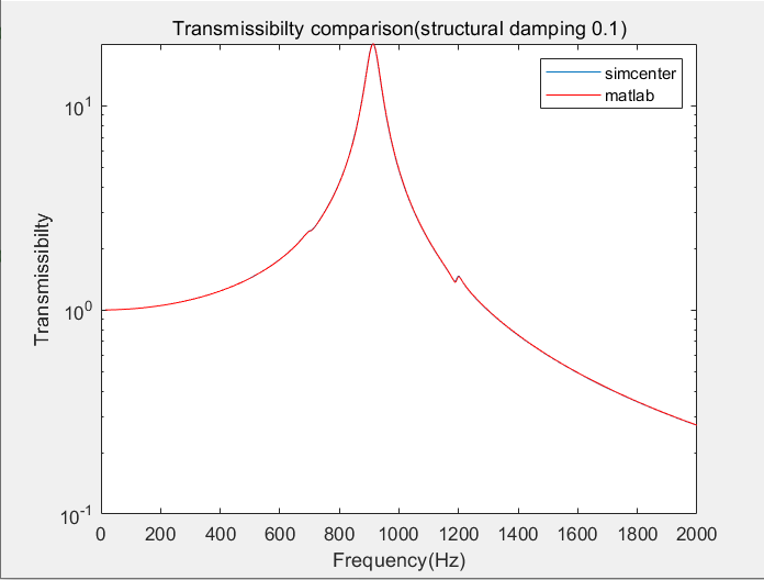
- structural damping이 10%인 경우
상대 오차 최대 0.24%
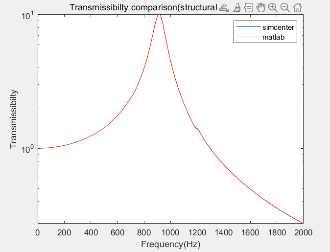
- structural damping이 5%인 경우
상대 오차 최대 0.26%
Cf) 주의 사항
Response Dynamics에서, base node 와 cbush를 RBE2 로 연결하면 다음과 같은 warning 메시지가 뜸
WARNING
Potential problems with the rigid links may exist in the model:
- Rigid Links are connected to elements which do not have rotational degrees of
freedom (DOF). This may result in solver errors.- Rigid Links connected to other rigid links. (Watch for rigid loops.)
- Rigid Links not connected to other elements.
If solver fails, check for inconsistent degrees of freedom.
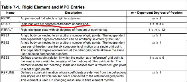
아래의 simcenter 1D rigid element 들 확인
- element 끝에 6자유도가 있는 RBAR 이용하기!!