본 코드는 'Week 14a: CNN and XGBoost Ensemble' 코드를 기반으로 작성되었습니다.How to spot a fake Nike Air Jordan?
진품과 가품은 미술 작품에서만 볼 수 있는 것이 아니다.
얼마전 삼성그룹 故 이건희 회장이 기증하여 현재 국립중앙박물관에 소장되어 있는 故 이중섭 작가의 황소 그림이다. 두 그림을 놓고 육안으로 보면 차이가 확연히 들어나는 것 처럼 보인다.
하지만, 시대가 변화고 기술이 발전하면서 미술작품 뿐만아니라, 사람들이 관심을 가지고 많이 찾는 것들은 항상 가품이 존재하기 마련이다.

무신사도 가품에 울었다…"냄새 맡는건 기본" 진짜찾기 전쟁
최근 명품의 중고 거래나 리셀(Resell, 재판매) 시장이 MZ세대들에게 뜨거운 관심을 받으며 백화점이나 상점 오픈 시간에 맞춰 줄을 서는 일명 오픈런을 보는 것은 흔한 광경이 되어버렸다.
무신사는 온라인으로 의류, 특히 국내,외 유명 브랜드를 판매 또는 유통하는 곳으로 널리 알려져있다. 유명 연예인들을 광고 모델로 내세우며 유명세를 이어가고 있고, 코로나 후 오갈데 없는 젊은 세대들의 뭉칫돈이 유명 브랜드 옷이나 악세사리 구매로 몰리며 연 매출이 눈에 띄게 증가하였다.
하지만 전문적으로 의류를 취급하는 무신사도 가품을 판매하며 곤욕을 치르기도 하였다.
국내에선 지난 2월 무신사와 네이버라는 거대 회사 두 곳이 맞붙은 가품 판매 논란이 있었다.
무신사에서 스트리트 패션 브랜드 '피어 오브 갓'의 로고 티셔츠를 구매한 한 소비자가 리셀
플랫폼 네이버 크림에 되팔기 위해 검수를 의뢰했으나, 크림에서 이를 가품으로 판정하고 판매를
거부한 것. 이후 무신사는 판매 제품을 들여온 해외의 티셔츠 판매처(팍선) 및 국내외 검증
전문기관의 정품 인증서 등을 증거로 제시하며 두 달간의 공방전이 이어졌다. 결과는 크림의 승.
“무신사의 판매 제품은 가품”이라는 피어 오브 갓 본사의 판정으로 크림은 이후 신뢰도가
높아지며 사용자가 급상승했다.
위 기사에서도 볼 수 있듯이, 유명 브랜드를 선호하는 젊은 층들 사이에서는 진품과 가품을 구분하는 일은 습득해야 하는 필수 스킬 중 하나가 되어버린 셈이다.
백화점 명품관 또는 편집샵 등 오프라인 공식 판매처에서 판매되고 있는 상품들은 소비자가 진품이라 믿고 구매하게 되지만, 여러 중고앱을 통한 개인 간 거래를 하거나 온라인을 통해 구매하게 될 경우 상품의 진위 여부를 스스로 판단하기 어렵다.
본 과제에서는 모든 연령 층에서 사랑 받고 있는 나이키 신발의 진위 여부를 알아보기 위해 classification task를 진행할 예정이다.
(1) 이미지 전처리
#(아래) 구글 검색 이미지 예시
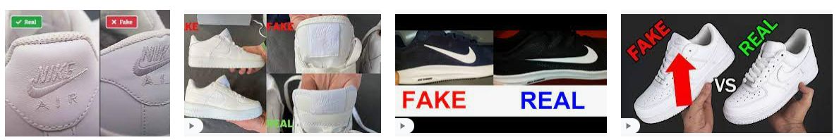 google에서 'nike real fake'로 검색 후 위와 같이 authentic or genuine nike 상품과 fake or counterfeit nike 상품이 구분된 이미지들을 선별하여 real과 fake 이미지들을 수작업으로 편집하고, 이후 별도 폴더에 저장하였다.
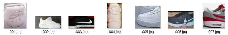
#(아래) 이미지 전처리 결과 예시 (real 이미지의 일부)
(2) 필요 라이브러리 import
### Important parameters

# random seed
my_seed = 42

# for creating color clusters, what % of pixels from each image are randomly sampled?
pixel_sample_perc = 0.2

# dropbox link for data
droplink = 'https://www.dropbox.com/s/dml1v6hafkfb6rf/nike.zip?dl=0'

# dropbox link zipfile name
drop_fn = 'nike.zip'

# dropbox local save folder name
drop_save_dir_nm = './nike'

# CNN image size and batch size
# image_size = (200, 200) # 별도로 계산하여 사용
batch_size = 2
(3) 학습 준비
여기서 image_size는 임의의 고정 값을 사용하지 않고, 전처리된 이미지 shape의 평균값을 활용하기로 하였다. Batch_size는 여러 실험 결과 2로 정하였다.
# Common imports
import os
import pandas as pd
import numpy as np
import cv2
import glob
import random

import tensorflow as tf
from tensorflow import keras
from tensorflow.keras import layers
import pathlib

import matplotlib.pyplot as plt

from fastai.vision.all import *
#from fastai.text.all import *
#from fastai.collab import *
#from fastai.tabular.all import *

from matplotlib.pyplot import imshow

from tensorflow.keras.utils import image_dataset_from_directory
from keras.preprocessing.image import ImageDataGenerator

!wget -O {drop_fn} {droplink}

!unzip {drop_fn} -d {drop_save_dir_nm}

# grab image list

img_list = glob.glob(drop_save_dir_nm + '/*/*.jpg')
img_list[0:10]

len(img_list)
182 # length of (img_list)
input 이미지들의 shape을 구하여, width 및 height의 평균 값을 계산 후 img_size 값으로 사용
from google.colab.patches import cv2_imshow

temp1 = []
temp2 = []

for i in range(len(img_list)):
  img = cv2.imread(img_list[i])
  # cv2_imshow(img)
  temp1.append(img.shape[:1]) # img shape의 width 값
  temp2.append(img.shape[1:2]) # img shape의 height 값

print(np.mean(temp1)) # img shape의 width 평균 값
print(np.mean(temp2)) # img shape의 height 평균 값
448.75824175824175 # image shape의 width 평균 값
600.8406593406594 # image shape의 height 평균 값img_size_new = np.minimum(np.mean(temp1), np.mean(temp2)) # img shape의 width, height 중 작은 값을 사용
print(img_size_new)
img_size_new = int(img_size_new) # integer로 변환
print(img_size_new)
# CUDA out of memory issue로 img_size를 반으로 줄여 다시 시도
img_size = (int(img_size_new/2), int(img_size_new/2)) # img_size로 사용
print(img_size)448.75824175824175
448
(224, 224) # img_size는 평균 값의 1/2 값을 사용
real과 fake 이미지의 총 개수는 182개로 real 91, fake 91개로 동일한 개수로 구성
# combine these lists as a dataframe

df = pd.DataFrame(list(zip(img_list, file_gid, file_label)), columns=['file_path', 'iid', 'label'])
df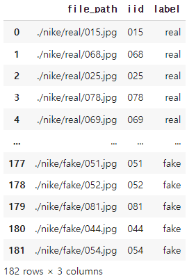
Label 생성
# create 0, 1 label

df.loc[df['label']=='fake', 'fake'] = 1
df.loc[df['label']=='real', 'fake'] = 0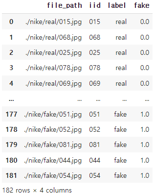
(4) CNN 학습
Train과 Valid set으로 나눈 후 먼저 CNN 학습
# data block settings

# for more information on datablock, please refer to:
# https://docs.fast.ai/tutorial.datablock.html

my_dblock = DataBlock(
    blocks=(ImageBlock, CategoryBlock),
    splitter=ColSplitter(), # split train and valid sets using 'is_valid'
    get_x=ColReader(0), # use image path from the first column of the df
    get_y=ColReader(3), # use label from the fourth column of the df
    item_tfms=Resize(img_size[0]))
# prepare dataloaders and show batch
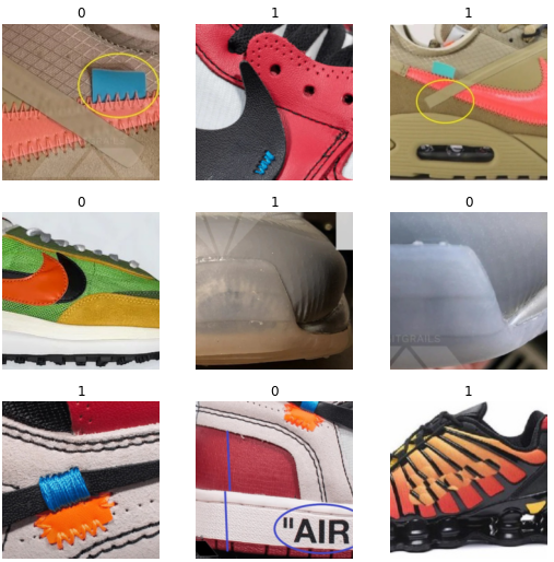
dls = my_dblock.dataloaders(img_combined_fastai)
dls.show_batch()아래는 batch 예시 (가품과 진품을 육안으로 구분하기 어렵다.)
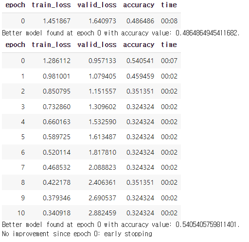
Early stopping, patience=10을 사용하여 학습을 진행하였다.
# with early stopping
learn_es = vision_learner(dls, resnet101, metrics=accuracy).to_fp16() # resnet 18, 34, 50, 101, 152
learn_es.path = Path('./early_stopping')

learn_es.fine_tune(30, cbs=[EarlyStoppingCallback(monitor='accuracy', patience=10),SaveModelCallback(monitor='accuracy')])
육안으로 구별하기 어려운 것처럼 accuracy도 높지 않다.
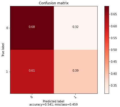
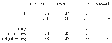
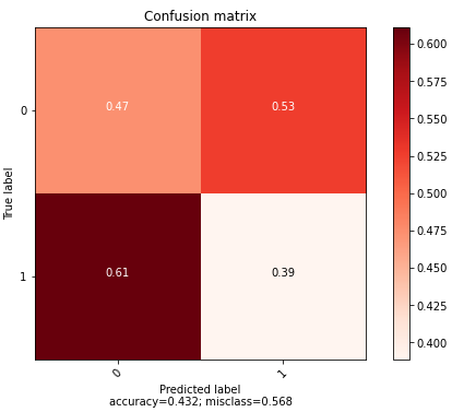
from sklearn.metrics import confusion_matrix, classification_report

print(classification_report(y_valid, y_pred_valid_cnn))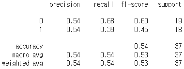
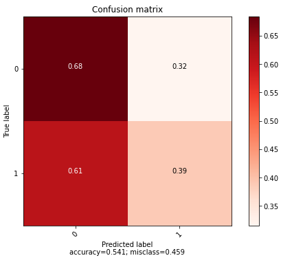
Confusion matrix 확인 결과 가품 구별을 잘 하지 못하는 것으로 보인다. Image augmentation을 해보았지만 accuracy가 향상되지 않았다.
(5) XGBoost 학습
다음은 XGBoost를 활용해 학습을 진행하였다.
%%time

early_stop_rounds = 10

# use early stopping

xgb_classifier.fit(df_palette_train, y_train,
            eval_set=[(df_palette_valid, y_valid)], early_stopping_rounds=early_stop_rounds)
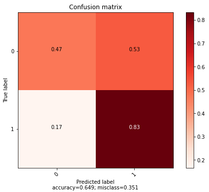
Loss를 보면 XGBoost도 마찬가지로 학습이 잘 되지 않는 것을 볼 수 있다.
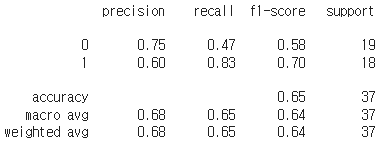
가품은 잘 맞추지만 진품은 잘 맞추지 못 하는 것을 볼 수 있다.
Randomized search CV를 활용해 최적화 진행 결과는 다음과 같다.
(6) Ensemble (CNN + XGBoost)
다음은 CNN과 XGBoost의 Ensemble 결과이다.
Accuracy가 좀 더 높은 CNN 쪽에 weight을 더 주고 학습하였다. 여러 실험을 진행하였지만, 6:4가 최적 값을 주었다.
# ensembled prediction

cnn_weight = 6
xgb_weight = 4

y_pred_valid_ensemble_proba = (cnn_weight*y_pred_valid_cnn_proba2 + xgb_weight*y_pred_valid_tuned_proba2)/(cnn_weight+xgb_weight)
y_pred_valid_ensemble_proba
(7) 결론
Ensemble 결과