.png)
8.1 The Basics of Decision Trees
8.1.1 Regression Trees
<Predicting Baseball Player's Salaries Using Regression Trees>
-
predictors : Years(메이저리그에서 몇년있었는지) / Hits(전년도의 Hits수)
-
reponse : Salary
-
Tree 구조 : Nodes(Terminal Nodes, Internal Nodes) / Splitting Ruels / branches
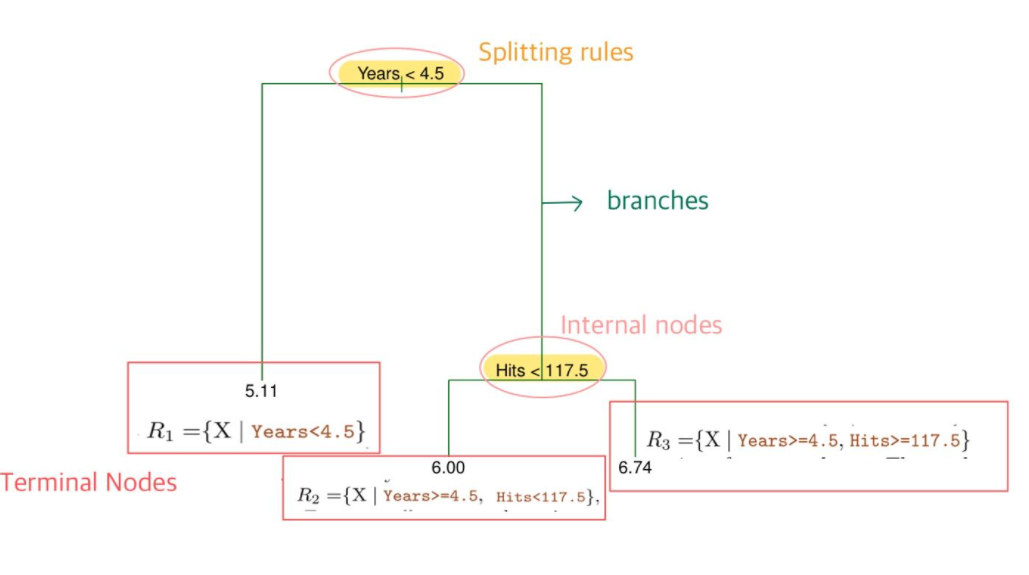
Terminal Nodes 를 수식으로 표현하면 위와 같이 R1,R2,R3의 Region으로 표현할 수 있음
<Predicting Baseball Player's Salaries Using Regression Trees>
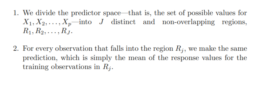
- Splitting Rules에 따라 데이터를 나누고
→ 최종 분리된 이후 예측값은 각 Ternimal Node (최종으로 분류되어 나온 Region)에 해당하는 mean response value for the training observations 로 함
(따라서, 같은 terminal Nodes에 있는 data들의 예측값으 모두 동일)
- 그럼 어떻게 Regions R1,R2,R3..Rj (Terminal Nodes, Tree 구조) 를 결정하는가?
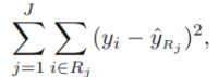
goal : find boxes R1,R2,R3..Rj that minimize the RSS
- Recursive binary Splitting
모든 경우의 수의 Splitting case를 전부 살펴볼 수 없기 때문에 top-down approach를 이용한다.
- RSS를 가장 작게하는 Predictor 와 적당한 Cutpoint를 지정하여 Splitting Rule을 만든다
HOW? 모든 Predictors와 그에 해당하는 모든 cutpoint를 고려한 뒤, lowest RSS를 가져다주도록 Splitting Rule을 결정
- 위와 같은 방법을 반복하여 , stopping criteria에 도달할 때까지 Split한다.
단. 전 단계에서 생성된 2개의 regions을 전부 split하는 것이 아닌, 두개 중 하나의 region만 Split한다.
Tree Pruning
- Tree가 너무 복잡해지면 Overfitting이 일어날 수 있음
- Smaller Tree (with fewer splits)은 lower variance 와 Better interpretation을 제공하지만, bias는 커진다.
적절한 tree structure는 어떻게 얻어내는가?
- 적절한 기준점(thresold)에 다다르면 tree split을 stop하는 방법론을 사용하여 ,적절하게 tree의 split 개수를 조정할 수 있음. (최소 RSS에 다다르지 않더라도)
→ 그러나 이렇게 단순한 방법으로 tree structure를 결정하면, 중요한 split rule이 뒤에 나오게 될 경우 RSS가 매우 커지는 단점이 있음.
- Tree Pruning : Tree의 Complexity는 낮추면서 동시에 RSS를 작게하기 위해 사용하는 방법
- Very Large Tree T0를 설정
- 적절한 Subtree (Test Error rate을 가장 작게 하는 → 이때 Test Error rate은 CV(Cross validation)을 이용하여 계산) 를 얻기 위해 prune it back(가지치기)
하지만 모든 subtree의 test error rate을 전부 계산할 수는 없음
→ selecting a samll set of subtrees for consideration : Cost Complexity pruning
- Cost Complexity pruning
: 모든 subtree를 계산하는 것이 아니라, 적절한 tuning parameter에 따라 결정된 subtree 후보 몇개만 살펴 보는 것
T : # of terminal tree (tree complexity)
a : tuning parameter
좌측 항 : RSS / 우측 항 : tree complexity에 대한 Penalty (a)
(a = 0이면, RSS를 최소로 하는 tree를 결정하면 되니까, T0를 선택하게 됨.
a 가 커질수록, Tree complexity에 대한 penalty는 커짐)
- CV를 이용해 test error rate이 가장 작아질 때의 a 값을 결정함 (tree complexity에 대한 penalty를 얼마나 줄 것인지 결정)
- a가 정해지면 그때 해당하는 subtree들을 이용하여 test error rate을 cv를 이용해 계산한 뒤 그 값이 가장 작아지는 tree를 선택함.
- Cost Complexity pruning 를 이용한 Tree stucture결정 알고리즘
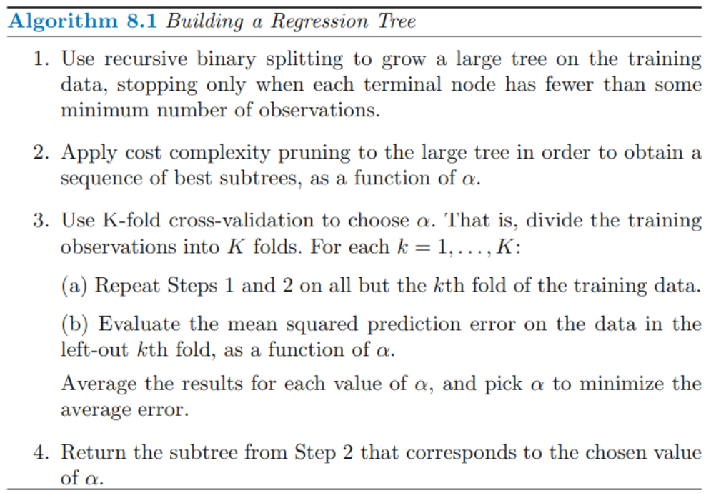
1 : 가장 큰 Tree를 만드는 것 (각 terminal node에 포함된 observations의 수가 some min number보다 작을 때)
2, 3 : pruning parameter값 결정
4 : final tree결정
8.1.2 Classifcation Trees
-
예측값 : 해당 Terminal Node에서 가장 빈도수가 높은 class of training observations 로 예측
(Most Commly occurring class)
-
RSS 대신 Classification error rate을 이용
<Classification error rate>
Most commonly occurring class (해당 Terminal Node에서 예측할 Class)에 속하지 못한 class의 비율
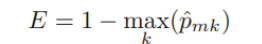
(Pmk : m번째 구역의 k번째 class의 비율)
tree-growing에 sensitive하지 않기 때문에, 뒤에 두개의 방법을 더 선호함
<Gini index (Gini impurity)>
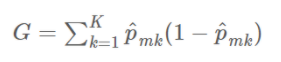
class가 덜 분류되어 덜 순수한 정도 반영
ex ) Class 가 2개 있는 경우 Pm1 = 1 , Pm2 =0 이어서 완벽히 분리된 경우 G는 0으로 계산된다.
Pm1 = 1/2 , Pm2 =1/2 이어서 반반 섞여 있는 경우, G는 0.5로 계산되어 값이 커지는 것을 알 수 있다.
→ Mth node가 pure(잘 분리되어 있을수록) small value를 가진다.
<Entropy>
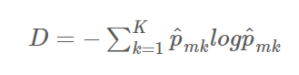
Gini index 와 거의 유사한 값을 가진다
분류 트리를 생성할 때는 gini impurity 혹은 entropy가 분기를 나누는 데에는 더 적합하여 주로 사용된다. 반면, 트리를 pruning 하는 작업에서는 정확도를 높이기 위해 classification error rate가 더 선호된다.
- tree model : predictors가 qualitative일 때도 사용가능
- Split했는데도 같은 predicted value를 줄 수 있음 → 그럼 왜 split하는가? node purity를 위해
한쪽 leaf이 보다 정확히 class를 분류하여 node purity를 증가시키는 경우 → test 에서의 정확한 분리를 위하여
8.1.3 Tree Versus Linear Models
linear model : features와 response의 관계가 linear일 때
tree model : non-linear and complex relationship btw features and response / 해석 및 시각화의 용이성이 필요할 때
8.1.4 Advantages and Disadvantages of Trees
Advantages
- explain하기 쉽다 (해석의 용이성)
- 사람의 decision rule과 비슷
- 시각화 하기 쉬움
- dummies 생성없이 범주형 변수 다루기 쉬움
Disdvantages
- same level of predictive accuracy 를 가지지 않음
- non-robust : data의 작은 변화에 크게 반응함
: High Variance
→ 문제 해결 : aggregating many decision trees
8.2 Bagging, Random Forests, Boosting, and Bayesian Additive Regression Tree
ensemble : simple building block model을 combining
8.2.1 Bagging
goal : Low varaince → averaging a set of observations reduce variance
여러개의 seperate training set을 이용해 얻어낸 값을 평균 내면 variance가 낮아짐
실제로는 train set을 여러개 얻기 어렵기 때문에
- Boostrap(Chap5)방법을 이용하여 bootstrapped training data sets을 얻고
- 각 training set에서 얻어진 predcitions을 평균낸다
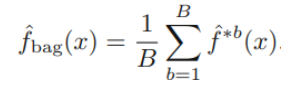
→ Bagging
tree에서 Bagging
- 각 tree B 는 deep and not pruned → high variance & low biase
- Averaging these B trees → reduce variance
B의 개수(single tree의 개수)는 overfitting 일으키지 않음
Out-of-Bag Error Estimaion
- 추출 되지 않아 (Boostrap되지 않아) training에 사용되지 않은 데이터 : Out-of-bag(OOB)
→ 이를 이용하여 Validation Test
-
전체 데이터 중 약 2/3정도가 한번의 Bootstarp에서 추출됨
-
B개의 single tree 중 i 번째 observation을 사용하지 않은 B/3개의 tree를 앙상블 하여 i번째 Observation에 대한 Validation Test 를 진행함
-
총 n개의 obervaion에 대해서 위와 같은 방법으로 prediction하면, overall OOB MSE / classification error를 얻을 수 있음
- cross-validation이 더욱 정확한 test error추정을 가능하게 하지만, 데이터가 충분히 많고 충분히 많은 B번의 Bootstrap의 경우 OOB 역시 비슷한 성능을 냄
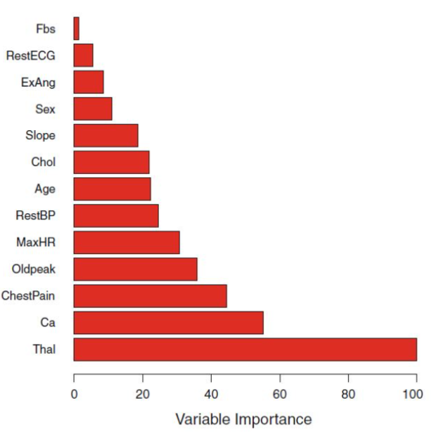
Variable Importance Measures
Bagging을 사용하면 model을 interpret하기 어려워지고, 어떤 variables가 tree building에 중요한 역할을 했는지 판별하기어려워짐
→ 이때, 각 tree에서 어떤 variables가 RSS 혹은 Gini Index를 줄이는데 일조했는지 record하고 가장 기여도가 높았던 순서대로 제시해줌으로써, Variable Importance 를 측정할 수 있게 해줌
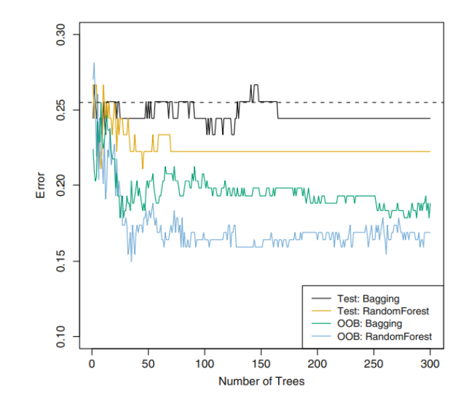
8.2.2 Random Forests
Bagging을 이용한다고 해도, 중요한 변수들은 고정되어있어 각 tree의 구조는 유사할 것이다
→ highly correlated trees
→ highly correlated quantites 들을 평균내는 것은 reduction Variance에 큰 도움이 안 됨
→ uncorrelated trees들이 필요 :
- 각 tree를 구성할 때, 전체 predictors 이용 대신 m개의 predictors만 고려하여 tree 구성.
- 각각의 tree는 m개의 변수만을 이용하게 되는데, 이때 변수의 importance를 고려해 m개를 고르는 것이 아니라, 단순하게 일부 개수의 변수만 사용함
그렇게 선택된 m개의 변수로 각 tree 구성 후, 평균을 내어 최종 예측 model이 구성됨
( m 의 개수는 일반적으로 p의 제곱근 : 그때 가장 성능 좋음)
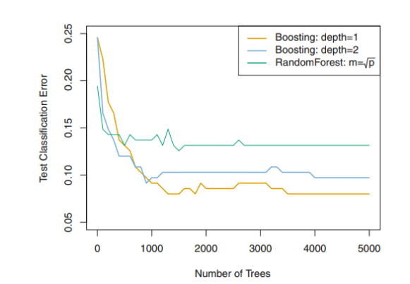
8.2.3 Boosting
Bagging과 유사하나, bootstrap sampling을 이용하지 않고 이전 tree 정보를 이용하여 sequentially grown 함.
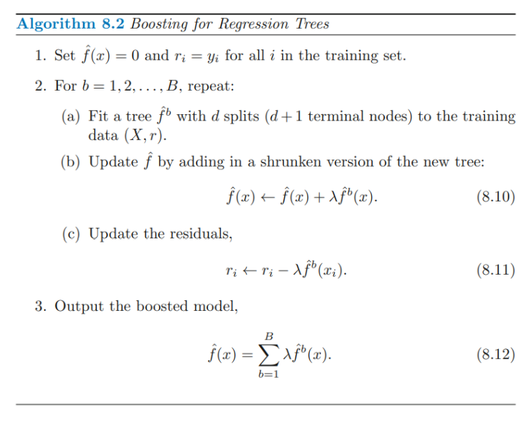
- Decision tree를 이전 model의 Residual에 fit : residual에 fit하기 때문에 small tree (d가 작음)
- Fitted function에 residual에 대한 정보를 update하기 위하여 1번에서 fit한 model의 결과를 더한다.
- residual을 update한다.
→ repeat하여 Fitted function 을 improving
: each tree depends strongly on the trees that have already been grown
Tuning Parameters
- The number of Trees : B
- Bagging , Random Forest와 다르게 B가 커지면 Overfitting됨
- B의 개수를 결정하기 위해서 CV사용
- shrinkaged parameter(lambda) : control the rate at which boosting learns
- 0.01 , 0.001
- B가 커지면 이 값이 작아져야 함
- The number d of splits in each tree : controls the complexity of the boosted ensemble
- d=1일 때 works well (stump)
8.2.5 Summary of Tree Ensemble Methods
Bagging
- 독립적으로 tree가 생성됨 따라서 각 tree는 모두 비슷
Random Forest
- bagging과 유사 but 모든 single tree가 유사해지는 것을 방지하기 위하여 각 single tree마다 random하게 predictors를 선택하여 tree를 생성함
Boosting
- Original data만 사용하고, random sample은 사용하지 않음
- 연속적으로 tree 생성 → slow learning approach
: current model이 설명해내지 못한 signal(residual)을 이용해 tree를 fit하고 이를 이용하여 fitted function을 update 시키고, 설명되지 않은 residual에서 설명된 부분 또한 update시킴