DFS

Directed Graph를 예시로 들어보자.
Graph가 adjacency list를 사용한다고 가정하자.

Setting of DFS

Color

• WHITE: 아직 discover 되지 않은 vertex

• GRAY: Discover 되었지만 아직 종료되지 않은 vertex

• BLACK: Discover 되고, 해당 vertex에 adjacency한 모든 vertex가 examine 된 vertex.

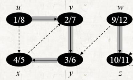
Timestamps

• $V.d$: discovery time

  • GRAY로 변한 시간

• $V.f$: finishing time

  • BLACK으로 변한 시간

Pseudo code of DFS

DFS(G)
1.  for each vertex u in G.V
2. 		u.color = WHITE
3.		u.π = NIL
4.  time = 0 //global variable
5.  for each vertex u in G.V
6. 		if u.color == WHITE
7.			DFS-VISIT(G, u)

Line 1 ~ 4: Initial setting
Line 5 ~ 7: 모든 vertex에 대해 탐색

DFS-VISIT(G, u)
1.  time = time + 1
2. 	u.d = time
3.  u.color = GRAY
4.  for each vertex v in G.Adj[u]
5. 		if u.color == WHITE
6.			v.π = u
7.			DFS-VISIT(G, v)
8.  u.color = BLACK
9.  time = time + 1
10. u.f = time

Line 1 ~ 2: discovery time setting
Line 4 ~ 7: adjacency vertex 탐색
Line 9 ~ 10: finishing time setting

DFS 특징

1. BFS와는 다르게 모든 vertex를 탐색한다.

   • 원래의 graph에서 connect 여부에 관계없이 사용가능하다.

2. 모든 vertex가 시작 vertex가 될 수 있다.

   • 모든 vertex가 WHITE로 초기화되어 있기 때문이다.

DFS 과정

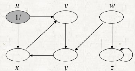
1. 한 vertex에 대해서 adjacency한 vertex를 탐색한다.

2. Adjacency한 vertex 의 $v.d, v.\pi, v.color$ = GRAY 를 세팅한다.

3. (2)에서의 vertex의 WHITE adjacency vertex를 확인한다.

4. 해당 vertex에 대해 (2) ~ (3) 과정을 반복한다.

5. 모든 Adjacency vertex를 확인했다면 처음 vertex의 다른 adjacency vertex에 대해 (2) ~ (4) 과정을 반복한다.

6. WHITE vertex가 남아있지 않을 때까지 (1) ~ (5) 과정을 반복한다.

7. 모든 vertex가 BLACK이라면 종료한다.

Running time of DFS

DFS(G)
1.  for each vertex u in G.V
2. 		u.color = WHITE
3.		u.π = NIL
4.  time = 0 //global variable
5.  for each vertex u in G.V
6. 		if u.color == WHITE
7.			DFS-VISIT(G, u)

DFS-VISIT(G, u)
1.  time = time + 1
2. 	u.d = time
3.  u.color = GRAY
4.  for each vertex v in G.Adj[u]
5. 		if u.color == WHITE
6.			v.π = u
7.			DFS-VISIT(G, v)
8.  u.color = BLACK
9.  time = time + 1
10. u.f = time

• Initializaion: $\theta(V)$

  • DFS(G)의 Line 1 ~ 4

• Graph Exploration: $\theta(V + E)$

  • DFS(G)의 Line 5 ~ 7
  • BFS와 다르게 $\theta$ 이다.
  • 방문하지 않는 vertex나 edge가 존재하지 않기 때문이다.
  • $= \displaystyle\sum_{i}^{X}\theta(V_i + E_i)$

• DFS-VISIT: $\theta(V_i + E_i)$

  • $V_i$: i번째 DFS-VIST에서 탐색할 vertex의 개수
  • $E_i$: i번째 DFS-VIST에서 탐색할 edge의 개수

• Total Running Time: $\theta(V + E)$

Depth - first forest

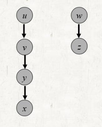
DFS에서의 predecessor subgraph는 forest이다.
Disconnected라는 점에서 BFS와 차이가 있다.

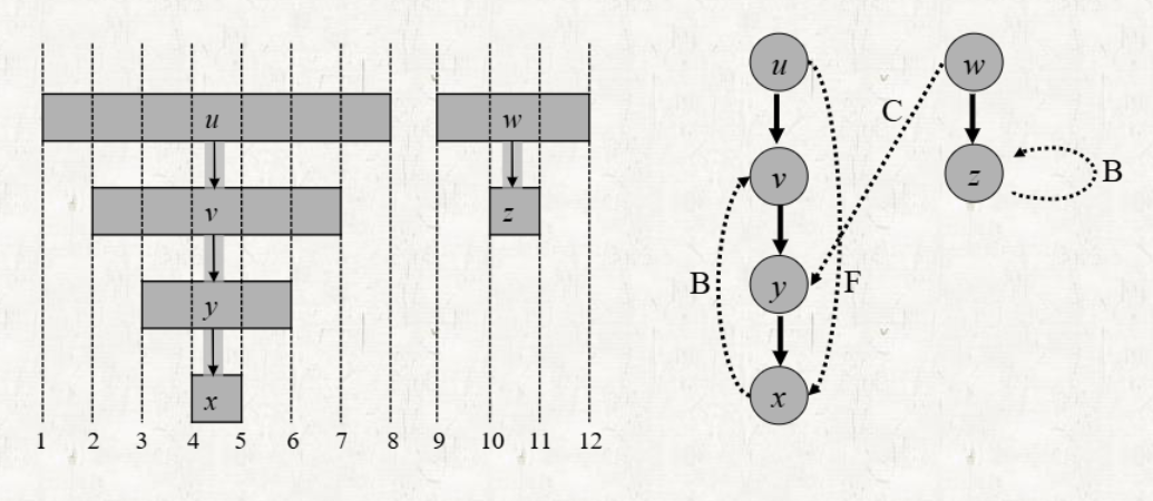
Parenthesis theorem for gray interval

Inclusion: Ancestor가 Descendant를 완벽하게 포함하는 경우

Disjoint: Inclusion이 아닌 경우

Overlap: Ancestor와 Descendant가 일부분만 겹치는 경우

• DFS에서는 Descendant가 종료되고 Ancestor가 종료되기 때문에 발생할 수 없다.

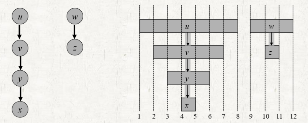
• u, v: disjoint
• u, y: Inclusion

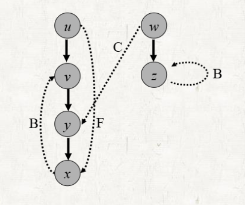
Classification of edges

1. Tree edges: forest 내에서 tree를 구성하는 edge

   • 아래 그림에서 실선에 해당한다.
   • Edges in a depth-first tree

2. Back edges: self loop / Descendant to Ancestor

   • Cycle을 형성한다.

3. Forwarding edges: Ancestor to Descendant

   • Tree edges는 제외된다.

4. Cross edges: 하나의 forest 내에서 서로 다른 tree의 vertex 간의 edge

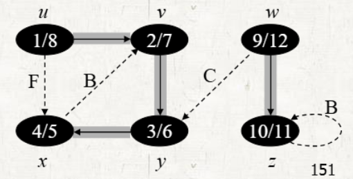
Classification of edges in DFS

edge (u, v)가 있다고 가정할 때, v의 color에 따라 edge가 분류될 수 있다.

• WHITE: tree edge

  • 아직 discover 되지 않은 vertex

• GRAY: back edge

  • GRAY라는 것은 한번 이상 discover 되었다는 것이기 때문에 v의 ancestor 이다.

• BLACK: forwarding or cross edge

  • Forwarding edge: $u.d < v.d < v.f < u.f$
  • Cross edge: $v.f < u.d$ 또는 $u.f < v.d$
  • 이처럼 v.color == BLACK인 경우에는 gray interval을 비교하여 정확히 분류할 수 있다.

• Edge의 종류를 결정할 때, constant time이 소요된다.

  • $u.d$ vs $v.d$ / $u.f$ vs $v.f$ 비교
  • color 이용하여 비교
  • Total Running Time에 영향을 미치지 않는다.

Example

DFS of undirected graph

Tree edge 와 Back edge 만 존재한다.

• Forwarding edge는 Back edge가 되고, Cross edge는 Tree edge가 된다.

• 이미 discover 된 정점 v를 만났을 때

  • 단순히 $v.\pi == u$ 의 여부만 확인하면 edge 종류를 결정할 수 있다.
  • Tree 종류를 결정하는데는 constant time이 소요된다.

Total Running Time

• 하나의 edge는 2개의 vertex에 adjacency 하다.
• $\theta(V + 2E)$ = $\theta(V + E)$