What is a Sorting Algorithm?

: 정렬 알고리즘은 입력으로 받은 일련의 리스트 혹은 배열의 값들을 특정한 순서를 통해 재배치하기 위한 방식을 말합니다. 일상생활에서 흔히 사용하는 오름차순, 내림차순 정렬이 정렬 알고리즘의 한 예시라고 할 수 있습니다. 이러한 정렬 알고리즘은 특히 DataBase에서 데이터를 CRUD를 할 때 다양한 방면으로 검색의 효율성을 올리거나 하는 작업 등에 사용이 되기 때문에 아주 중요한 개념 중 하나라고 할 수 있습니다

Branchs of Sorting Algorithms

• Selection sort
• Bubble sort
• Insertion sort
• Merge sort
• Quick sort
• Heap sort
• Counting sort
• Radix sort
• Bucket sort

이렇게 크게 9가지의 범용적으로 사용되는 알고리즘이 존재합니다. 이러한 알고리즘도 특정 조건에 따라서 구분을 하여 사용할 수 있습니다.

1. 숫자의 교환 또는 변환이 필요할 때
2. 숫자를 비교할 때
3. 재귀식을 사용하거나 하는 경우
4. 안정하거나 안정하지 않은 경우
5. 추가적인 저장 공간이 필요한 경우

Bucket Sort

: Bucket Sort는 비교를 위해서 각 요소들을 나누고 해당하는 바구니에 담아서 그 각각의 바구니를 정렬하는 정렬 알고리즘 입니다. 해당 알고리즘은 주로 균일한(Uniformly) 범위에 걸쳐 분포되어 있을 때 사용됩니다. 이러한 로직을 통해 분리된 버켓은 merge sort, heap sort, quick sort, insertion sort 과 같은 알고리즘에 의해 분류 되었을 때 시간 복잡도는 Big-O notation으로 표현하면 O(nlogn) 으로 나타낼 수 있습니다. 만약 그 안의 원소를 정렬하지 않고 그대로 출력 할 경우에는 O(n) 입니다.

---

Counting Sort

: Counting sort는 먼저 개수 혹은 고유한 값의 발생에 대한 리스트를 만듦으로써 동작하게 됩니다. 해당 과정을 거침으로써, 최종적으로는 개수에 관한 리스트를 기반으로 생성이 됩니다. 해당 정렬은 리스트 안의 범위를 알고 있을 때 사용이 됩니다.

Say you have a list of integers from 0 to 5:
 
input = [2, 5, 3, 1, 4, 2]

First, you need to create a list of counts for each unique value in
the `input` list. Since you know the range of the `input` is from 0 to
5, you can create a list with five placeholders for the values 0 to 5,
respectively:

count = [0, 0, 0, 0, 0, 0]
  # val: 0  1  2  3  4  5

Then, you go through the `input` list and iterate the index for each value by one.

For example, the first value in the `input` list is 2, so you add one
to the value at the second index of the `count` list, which represents
the value 2:

count = [0, 0, 1, 0, 0, 0]
  # val: 0  1  2  3  4  5
       
The next value in the `input` list is 5, so you add one to the value at
the last index of the `count` list, which represents the value 5:

count = [0, 0, 1, 0, 0, 1]
  # val: 0  1  2  3  4  5

Continue until you have the total count for each value in the `input`
list:

count = [0, 1, 2, 1, 1, 1]
  # val: 0  1  2  3  4  5

Finally, since you know how many times each value in the `input` list
appears, you can easily create a sorted `output` list. Loop through
the `count` list, and for each count, add the corresponding value
(0 - 5) to the `output` array that many times.

For example, there were no 0's in the `input` list, but there was one
occurrence of the value 1, so you add that value to the `output` array
one time:

output = [1]

Then there were two occurrences of the value 2, so you add those to the
`output` list:

output = [1, 2, 2]

And so on until you have the final sorted `output` list:

output = [1, 2, 2, 3, 4, 5]

위와 같은 output이 나올 경우에 Property는 아래와 같습니다

• Space Complexity : O(k)
• Best case performance : O(n+k)
• Average case performance : O(n+k)
• Worst case performance : O(n+k)
• Stable : Yes (k는 배열 안의 요소에 범위를 나타냅니다.)

---

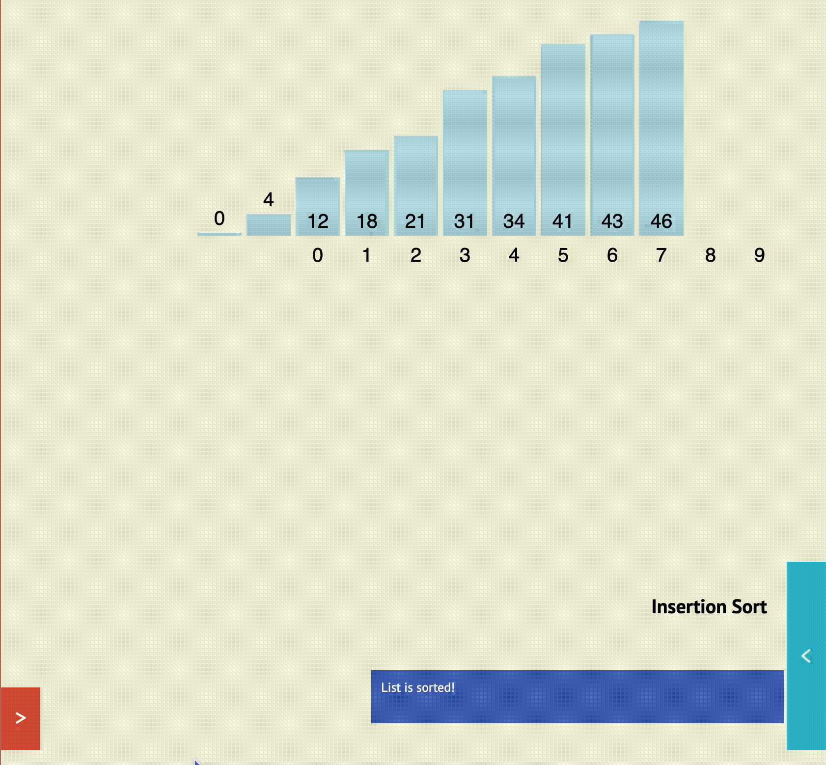
Insertion Sort

: Insertion Sort은 간단하게 크기 순으로 비교하여 나열하는 알고리즘이다. 즉, 첫 인덱스에 있는 요소를 시작으로 비교를 하여 순서를 서로 바꾸고 업데이트를 하며 정렬을 하는 방식이다.

public int[] insertionSort(int[] arr)
      for (j = 1; j < arr.length; j++) {
         int key = arr[j]
         int i = j - 1
         while (i >= 0 and arr[i] > key) {
            arr[i+1] = arr[i]
            i -= 1
         }
         arr[i+1] = key
      }
      return arr;

Insertion sort 알고리즘을 통해서 정렬을 할 경우의 Properties는 Big-O notation으로 표현 할 경우 아래와 같다.

• Space Complexity : O(1)
• Time Complexity : O(n), O(nn), O(nn) → 해당 상황은 최적의 결과와 평균적인 결과, 그리고 최악의 경우를 보여줍니다.
• Best Case : 배열이 이미 정렬이 되어 있는 경우
• Average Case : 배열이 랜덤하게 정렬이 되어 있는 경우
• Worst Case : 거꾸로 배열이(역순으로) 정렬이 되어 있는 경우

Merge Sort

Merge Sort는 분할과 정복을 통해서 정렬을 하는 알고리즘 입니다. 배열의 요소를 쪼개어 다시 합병 시켜 나가는 과정에서 다시 재정렬을 해나가는 방식을 사용하고 있어 Quick Sort와 유사한 방식을 가지고 있음을 알 수 있습니다.

• 풀이 과정

1. 리스트의 길이가 0 또는 1이면 이미 정렬된 것으로 봅니다.
2. 그렇지 않은 경우, 정렬되지 않은 리스트를 절반으로 잘라 비슷한 크기의 두 부분 리스트로 나눈다.
3. 각 부분 리스트를 재귀적으로 합병 정렬을 이용해 정렬한다.
4. 두 부분 리스트를 다시 하나의 정렬된 리스트로 합병한다.

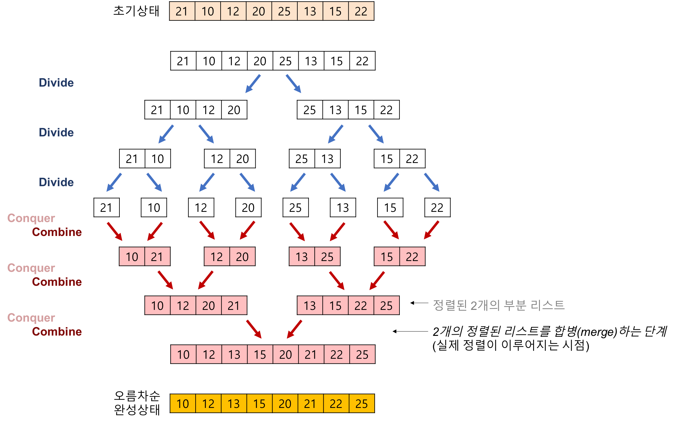
• 예시)
  

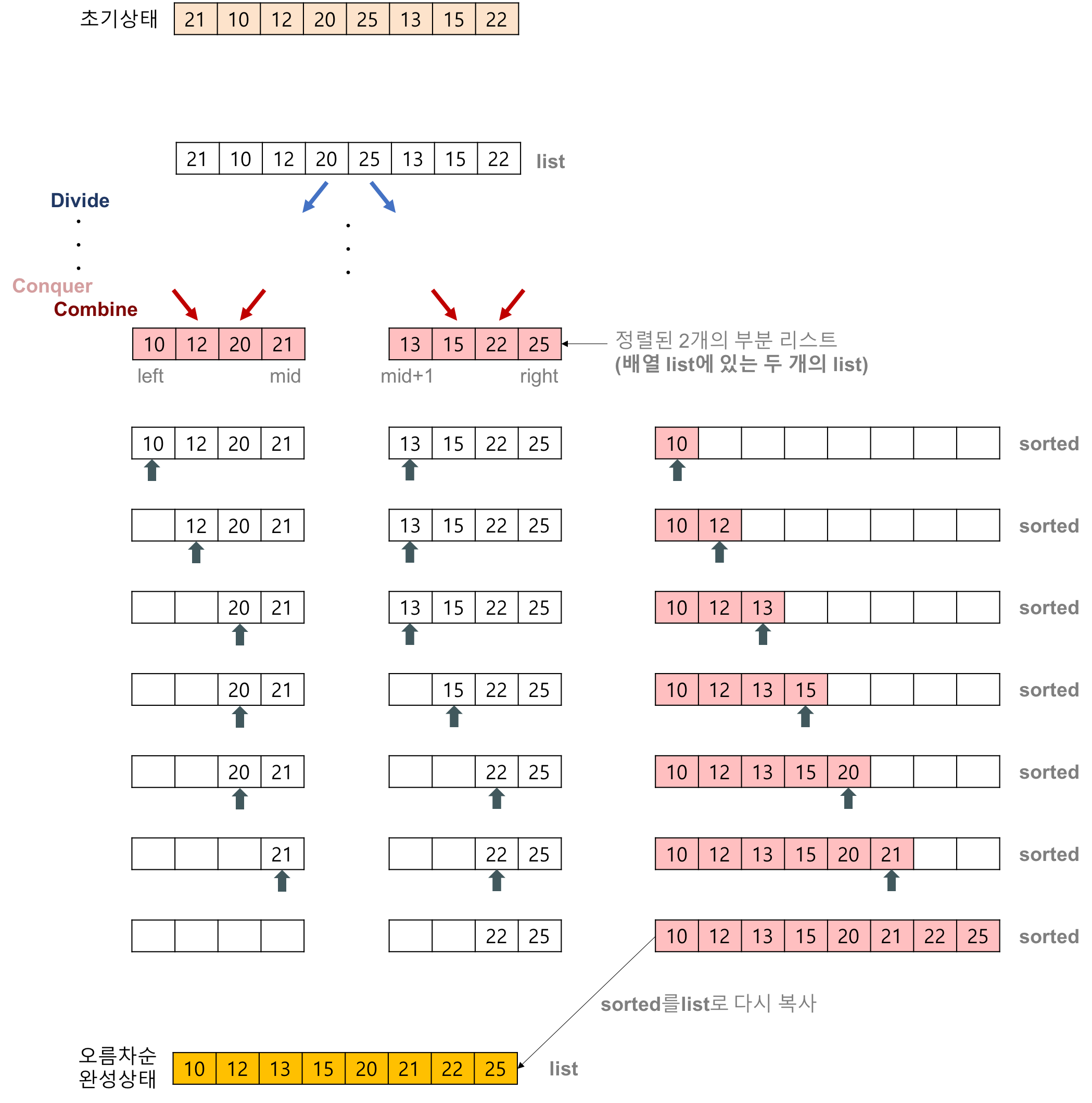
Merge Sort도 Quick Sort에서 말한 것과 같이 Devide, Conquer, Combine 이 세과정을 거쳐서 정렬이 되는 것으로 볼 수 있다.

Pinpoint of Merge Sort

• Strength

1. Merge Sort는 데이터 분포에 영향을 덜 받기 때문에, 어떤 데이터든 정렬되는 시간은 동일하게 가져 올 수 있다. → O(nlog₂n)
2. 만약 레코드를 Linked List로 구성한다면, 연결된 인덱스만 변경되므로 데이터의 이동은 무시할 수 있을 정도로 작아져 In-place-sorting을 구현 할 수 있다.
3. Weakness를 보완하기 위해서 대량의 레코드를 정렬할 때 는 연결 리스트를 구현하여 하는 것이 다른 정렬들 보다 효율적이다.

• Weakness

1. 만약 레코드를 배열로 구성하면, Merge Sort는 in-place sorting이 아니기 때문에 임시배열이 필요하여 레코드의 개수가 많아지게 될 경우 이동 횟수가 많아져 큰 시간적 낭비를 가져올 수 있다.

private void solve() {
    int[] array = { 230, 10, 60, 550, 40, 220, 20 };
 
    mergeSort(array, 0, array.length - 1);
 
    for (int v : array) {
        System.out.println(v);
    }
}
 
public static void mergeSort(int[] array, int left, int right) {
    if (left < right) {
        int mid = (left + right) / 2;
 
        mergeSort(array, left, mid);
        mergeSort(array, mid + 1, right);
        merge(array, left, mid, right);
    }
}
 
public static void merge(int[] array, int left, int mid, int right) {
    int[] L = Arrays.copyOfRange(array, left, mid + 1);
    int[] R = Arrays.copyOfRange(array, mid + 1, right + 1);
 
    int i = 0, j = 0, k = left;
    int ll = L.length, rl = R.length;
 
    while (i < ll && j < rl) {
        if (L[i] <= R[j]) {
            array[k] = L[i++];
        } else {
            array[k] = R[j++];
        }
        k++;
    }
 
    while (i < ll) {
        array[k++] = L[i++];
    }
 
    while (j < rl) {
        array[k++] = R[j++];
    }
}

Heap Sort

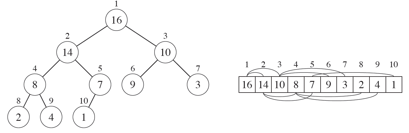
Heap 이란?

트리 구조를 기반으로 하는 자료 구조중 하나로써, Higher Key(우선 순위)에 자주 액세스하거나 Key(우선 순위) 중심으로 정렬된 시퀸스를 활용해야 할 때 유용한 자료구조 입니다. 한 node가 최대 두 개의 child node를 가지면서, 마지막 레벨을 제외한 모든 레벨에서 노드들이 꽉 채워진 Complete Binary tree를 기본으로 합니다.

💡 Binary Tree란?
이진 트리 구조는 크게 Full Binary Tree & Complete Binary Tree, Balanced Binary Tree 등이 있습니다.

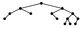
• Full Binary Tree
  
  On this Structure, it has a shape of tree in which every node has either 0 or 2 child node and All leaves node are at the same level.
• Complete Binary Tree
  
  Like a slightly different from a case of above, aComplete Binary Tree is a tree in which every level, except possibly the last, is completely filled, and all nodes are as left as possible. In addition, We are also able to describe this tree model into the 1 demensional array.
  
• Balanced Binary Tree
  Balanced Binary Tree는 예측 가능한 깊이(Predictable depth)를 기자며, node가 n인 log(n)을 내림한 값이 됩니다.
  
  A Balanced Binary Tree has a shape in which the height of the left and right subtrees of any node differs by at most one and, this ensures that the tree is approximately balanced. Kind of Sorting algorithm like Insertion, Deletion, Search can be performed efficiently.

• Heap order property : 각 노드의 값은 자신의 자식노드가 가진 값보다 크거나 같다(Max Heap). 각 노드의 값은 자신의 자식노드가 가진 값보다 작거나 같다(Min Heap).
• Heap shape property : Heap Sort의 data structure는 완전이진트리입니다. 즉, 마지막 레벨의 모든 노드는 왼쪽에 쏠려 있음을 알 수 있습니다.

Heap vs Binary Search Tree

This picture refers to the Binary Search Tree Structure now. Heap and Binary Search Tree commonly have a point that shares what we can look out. but if we look trought inside in it, they seemed to be a bit having each differential points.

Heap has noramlly higher value than a root node in which is on the left from the root node and the right node will be higher than node. So, this algorithm has a advantages for priority soring and binary search tree.

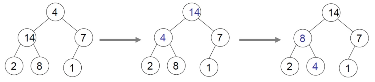
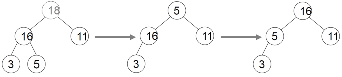
Heapify ↺

Showing below this line, make some array to be heapified, we should swap numbers like [4,10] -> [10,4].

import java.util.Arrays;

public class HeapifyExample {
    public static void main(String[] args) {
        int[] array = {4, 10, 3, 5, 1};

        System.out.println("Original Array: " + Arrays.toString(array));

        // Perform heapify
        heapify(array);

        System.out.println("Heapified Array: " + Arrays.toString(array));
    }

    // Heapify function
    static void heapify(int[] arr) {
        int n = arr.length;

        // Start from the last non-leaf node and heapify each node
        for (int i = n / 2 - 1; i >= 0; i--) {
            heapifyUtil(arr, n, i);
        }
    }

    // Heapify utility function
    static void heapifyUtil(int[] arr, int n, int i) {
        int largest = i;
        int left = 2 * i + 1;
        int right = 2 * i + 2;

        // Compare with left child
        if (left < n && arr[left] > arr[largest]) {
            largest = left;
        }

        // Compare with right child
        if (right < n && arr[right] > arr[largest]) {
            largest = right;
        }

        // If the largest is not the root, swap and heapify the affected subtree
        if (largest != i) {
            int temp = arr[i];
            arr[i] = arr[largest];
            arr[largest] = temp;

            // Recursively heapify the affected subtree
            heapifyUtil(arr, n, largest);
        }
    }
}

• Time Complexity : O(log n)

• This is also kind of Data structure, So, it needs to be able to be possible insert iteration.
  
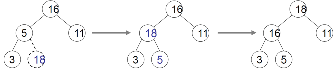
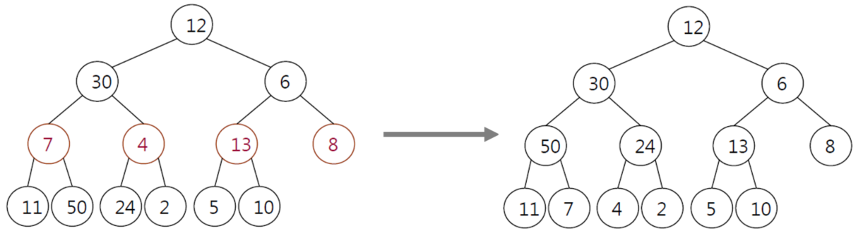
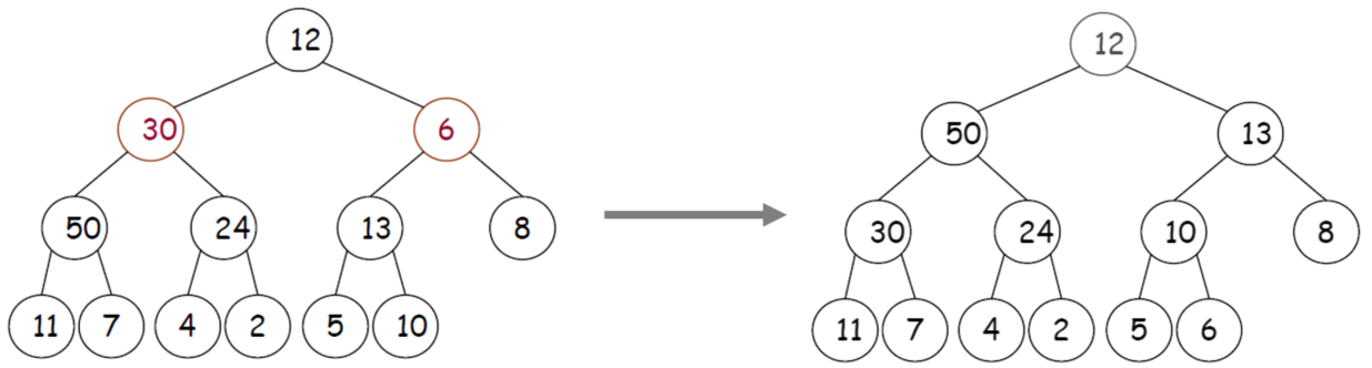
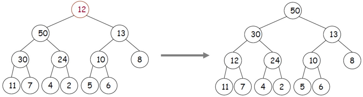
  Like above, we can look out the rule in the heap was broken. Now, applying the way of heapify It can be set up with the correct form. Lastly, we have to do heapify this tree from down to the top. Plus, we don't need to compare among the same level node value during heapifying. (T/C : O(log n) )

• Delete iteration
  

• Build Heap
  Build heap means to make some random value of MAX HEAP
  
  
  
  -> Time Complexity : O(n log n)

Radix Sort

Quick Sort, MergeSort, HeapSort 알고리즘은 기본적으로 비교를 통한 정렬을 하고 있습니다. 그에 반해 이 Radix Sort의 전제조건으로 오는 Counting Sort는 O(n+k)라는 시간 복잡도를 가지고 있습니다. 우리가 입력으로 오는 변수의 최소 자리수 혹은 판별에 유의미하다고 정의된 자리수의 숫자를 통해서 해당 숫자 혹은 문자가 입력 값에 얼마나 있는지 카운팅을 하는 것에 목적을 둔 알고리즘 입니다.

• Examples

int[] arr = {10, 21, 17, 34, 44, 11, 654, 123};

Radix_Sort_for_one(arr);

0: 10
1: 21 11
2:
3: 123
4: 34 44 654
5:
6:
7: 17
8:
9:

그리하여, 배열은 {10,21,11,123,34,44,654,17} 순으로 나열이 되게 된다. 이러한 과정을 자릿 수 별로 진행을 하게 되면 크기에 맞춰서 오름차순의 결과를 얻을 수 있다.

import java.util.Arrays;

public class RadixSortExample {
    public static void main(String[] args) {
        int[] array = {170, 45, 75, 90, 802, 24, 2, 66};

        System.out.println("Original Array: " + Arrays.toString(array));

        // Perform Radix Sort
        radixSort(array);

        System.out.println("Sorted Array: " + Arrays.toString(array));
    }

    // Radix Sort function
    static void radixSort(int[] arr) {
        // Find the maximum number to determine the number of digits
        int max = getMax(arr);

        // Perform counting sort for every digit place
        for (int exp = 1; max / exp > 0; exp *= 10) {
            countingSort(arr, exp);
        }
    }

    // Counting Sort function for a specific digit place (exp)
    static void countingSort(int[] arr, int exp) {
        int n = arr.length;
        int[] output = new int[n];
        int[] count = new int[10];

        // Initialize count array
        Arrays.fill(count, 0);

        // Store count of occurrences in count[]
        for (int i = 0; i < n; i++) {
            count[(arr[i] / exp) % 10]++;
        }

        // Change count[i] so that count[i] contains the actual position of the digit in output[]
        for (int i = 1; i < 10; i++) {
            count[i] += count[i - 1];
        }

        // Build the output array
        for (int i = n - 1; i >= 0; i--) {
            output[count[(arr[i] / exp) % 10] - 1] = arr[i];
            count[(arr[i] / exp) % 10]--;
        }

        // Copy the output array to arr[], so that arr[] now contains sorted numbers according to the current digit
        System.arraycopy(output, 0, arr, 0, n);
    }

    // Utility function to get the maximum value in the array
    static int getMax(int[] arr) {
        int max = arr[0];
        for (int value : arr) {
            if (value > max) {
                max = value;
            }
        }
        return max;
    }
}

Selection Sort

Selection Sort는 가장 단순한 알고리즘 중 하나입니다. 단순하게 배열에 있는 숫자들을 뽑아서 그것을 연산하고 자리를 바꾸는 형식으로 진행이 됩니다.

1. 배열 내의 가장 작은 숫자를 찾아 첫 요소와 위치를 바꾼다.
2. 위와 비슷한 과정을 반복한다.

public void selectionsort(int array[])
{
    int n = array.length;            //method to find length of array 
    for (int i = 0; i < n-1; i++)
    {
        int index = i;
        int min = array[i];          // taking the min element as ith element of array
        for (int j = i+1; j < n; j++)
        {
            if (array[j] < array[index])
            {
                index = j;
                min = array[j];
            }
        }
        int t = array[index];         //Interchange the places of the elements
        array[index] = array[i];
        array[i] = t;
    }
}

Bubble Sort🫧🫧

public class BubbleSort {
    static void sort(int[] arr) {
        int n = arr.length;
        int temp = 0;
         for(int i=0; i < n; i++){
                 for(int x=1; x < (n-i); x++){
                          if(arr[x-1] > arr[x]){
                                 temp = arr[x-1];
                                 arr[x-1] = arr[x];
                                 arr[x] = temp;
                         }

                 }
         }

    }
    public static void main(String[] args) {

		for(int i=0; i < 15; i++){
			int arr[i] = (int)(Math.random() * 100 + 1);
		}

                System.out.println("array before sorting\n");
                for(int i=0; i < arr.length; i++){
                        System.out.print(arr[i] + " ");
                }
                bubbleSort(arr);
                System.out.println("\n array after sorting\n");
                for(int i=0; i < arr.length; i++){
                        System.out.print(arr[i] + " ");
                }

        }
}

Properties

• Space Complexity : O(1)
• Best case Performance : O(n)
• Average case Performace : O(n*n)
• Worst case Performance : O(n*n)
• Stable : Yes

🌟 Quick Sort 🌟

Quick Sort 알고리즘은 효율적인 분할 및 정복 정렬 알고리즘 입니다.

• Quick Sort의 단계

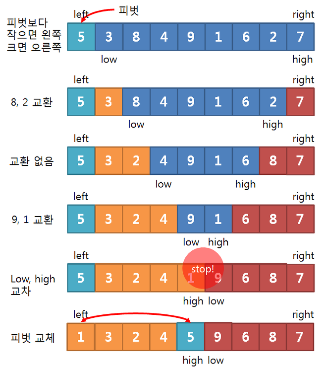
1. Divide : 입력 배열을 피벗을 기준으로 비균등하게 2개의 부분 배열(피벗을 중심으로 왼쪽 = 피벗보다 작은 요소들, 오른쪽 = 피벗보다 큰 요소들)로 분할합니다.

    static int partition(int[] arr, int low, int high) {
        int pivot = arr[low];
        int left = low + 1;
        int right = high;

        while (left <= right) {
            // Find element larger than the pivot in the left
            while (left <= right && arr[left] <= pivot) {
                left++;
            }

            // Find element smaller than the pivot in the right
            while (left <= right && arr[right] > pivot) {
                right--;
            }

            // Swap the elements found in the left and right
            if (left <= right) {
                int temp = arr[left];
                arr[left] = arr[right];
                arr[right] = temp;
            }
        }

        // Swap pivot with the element at the right pointer
        int temp = arr[low];
        arr[low] = arr[right];
        arr[right] = temp;

        return right;
    }
}

2. Conquer : 부분 배열을 정렬합니다. 부분 배열의 크기가 충분히 작지 않으면 재귀 함수를 이용하여 다시 분할 정복 방법을 적용합니다.

   static void quickSort(int[] arr, int low, int high) {
        if (low < high) {
            int pivotIndex = partition(arr, low, high);

            quickSort(arr, low, pivotIndex - 1);
            quickSort(arr, pivotIndex + 1, high);
        }
    }

3. Combine : 정렬된 부분 배열들을 하나의 배열에 합병합니다. 순환 호출(Recursion)이 한번 진행될 때마다 최소한 하나의 원소는 최종적으로 위치가 정해지므로, 이 알고리즘은 반드시 끝난다는 것을 보장 할 수 있습니다.

public class QuickSort {
    public static void main(String[] args) {
        int[] array = {23, 2, 26, 3, 12, 16};

        System.out.println("Original Array: " + Arrays.toString(array));

        quickSort(array, 0, array.length - 1);

        System.out.println("Sorted Array: " + Arrays.toString(array));
    }

Improvement of Quick Sort

Partition() 함수에서 피벗 값이 최소나 최대 값으로 지정되어 파티션이 나누어 지지 않았을 경우, O(n*n)이라는 시간 복잡도를 가지게 됩니다. 이러한 문제점을 개선하기 위해서 배열에 가장 앞에 있는 값과 중간 값을 교환해준다면 확률적으로나마 시간복잡도 O(nlog₂n)으로 개선 할 수 있습니다.

Best Case

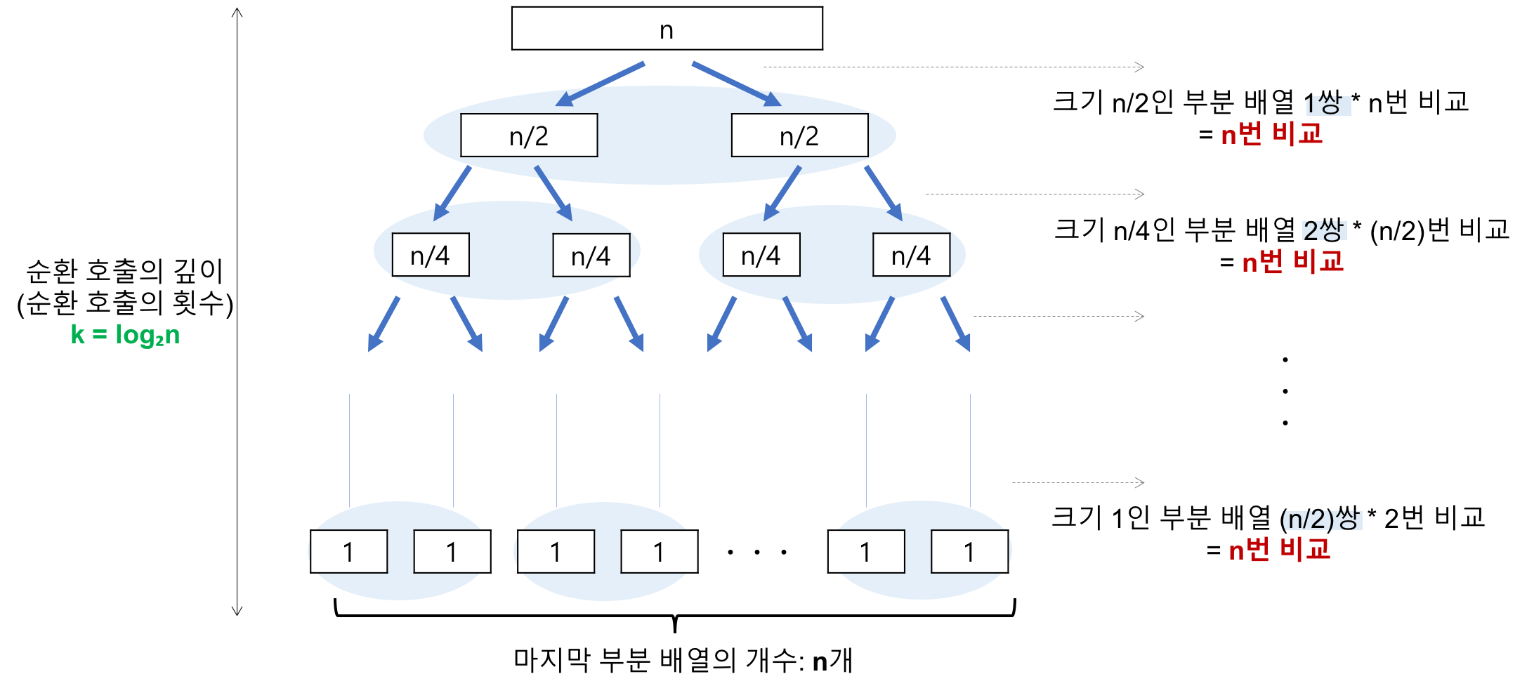
• T(n) = O(nlog₂n)
  레코드의 개수 n이 2의 거듭제곱이라고 가정(n= 2*k)했을 때, k가 3일 경우 점점 줄어 2의 0제곱까지 도달하게 됩니다. 그러한 과정에 의해서 해당 Recursion의 깊이가 3임을 알 수 있습니다.

위 내용을 일반화를 진행하면, n = 2^k의 경우, k(k=log₂n) 임을 알 수 있습니다.

Worst Case

• T(n) = O(n*n)
  최악의 경우는 위에서 말한 것과 같이 배열이 오름차순 정렬되어 있거나, 내림차순 정렬되어 있는 경우입니다.

Strength & Weakness
💡 불필요한 데이터의 이동을 줄이고 먼 거리의 데이터를 교환할 뿐만 아니라, 한 번 결정된 피벗들이 추후 연산에서 제외되는 특성 때문에, 시간 복잡도가 같은 O(nlog₂n)를 가지는 다른 정렬 알고리즘과 비교했을 때도 가장 빠르다.
💡 이미 할당 받은 저장공간 안에서의 정보 교환이기 때문에, 다른 메모리 공간을 필요로 하지 않는다.

💣 Unstable Sort입니다.
💣 정렬된 배열에 대해서는 Quick Sort의 Unstable Sort에 의해서 오히려 수행시간이 더 많이 걸리게 됩니다.

Tim Sort(Stable)

Tim Sort는 가장 빠른 알고리즘으로도 알려져 있는 stable하고 시간 복잡도는 평균적으로 O(Nlog(N))을 가지고 있습니다.

Tim Sort는 Merge Sort 와 Insertion Sort를 조합하여 사용하는 안정적이고 효율적인 정렬 알고리즘 입니다. 이러한 정렬 알고리즘은 Java의 Array.sort, Collections.sort, Python's Sorted()에 적용되어 있습니다. 각각의 시간 복잡도는 평균을 가정했을 경우, O(n^2)과 O(nlogn)임을 알 수 있는데 시간복잡도에 따른 빠르기를 계산해 보겠습니다.

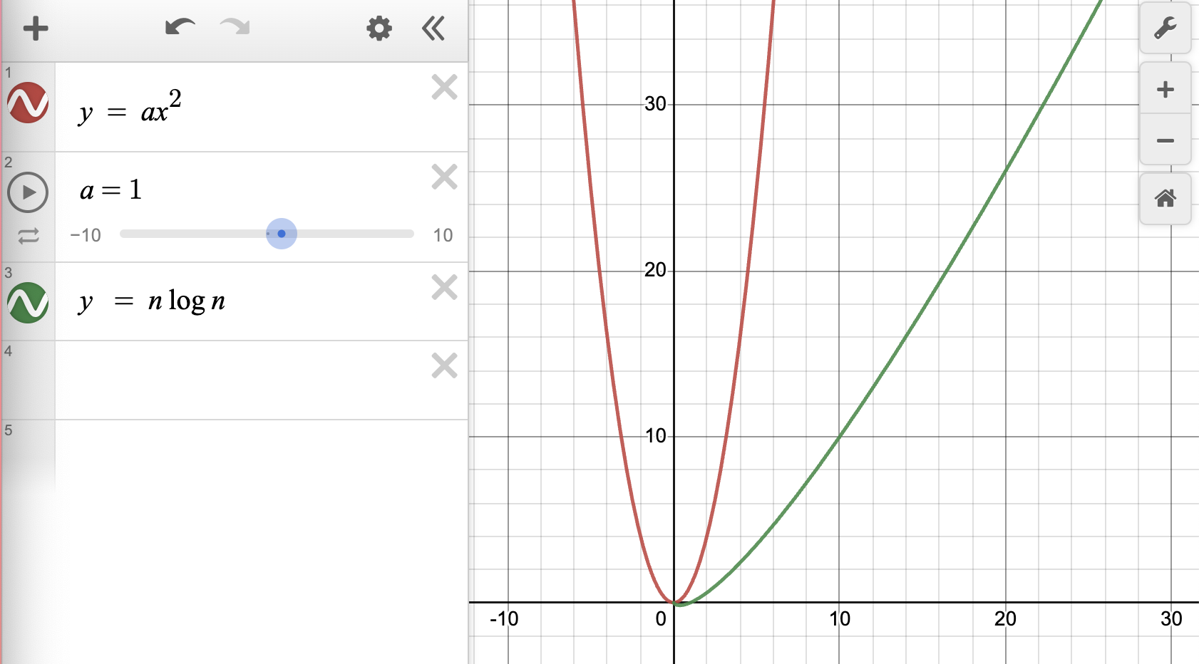
위의 사진으로 알 수 있다 싶이 기울기가 nlogn 그래프의 기울기가 훨씬 가팔라 속도가 느림을 확인 할 수 있습니다. 즉, Insertion Sort가 빠름을 알 수 있습니다. 이를 이용하여, 전체를 작은 덩어리로 각각 잘라서 Insertion Sort로 정렬 후 병합하는 것이 Tim Sort의 시작입니다.

배열이 N개 있을 때 2^x개씩 잘라 각각을 Insertion Sort를 통해서 정렬을 하면 Merge Sort보다 덩어리별 x개의 병합 동작이 생략되어, Merge Sort의 동작 시간을 C_m * n(log(n - x)) + a가 됩니다. 이때 x 값을 최대한 크게 하고 a값을 최대한 줄이기 위해 여러가지 최적화 기법이 사용됩니다.

• Part of Insertions Sort

static void insertionSort(int[] arr, int left, int right) {
    for (int i = left + 1; i <= right; i++) {
        int key = arr[i];
        int j = i - 1;

        while (j >= left && arr[j] > key) {
            arr[j + 1] = arr[j];
            j--;
        }

        arr[j + 1] = key;
    }
}

• Part of Merge Sort

static void merge(int[] arr, int left, int mid, int right) {
    int len1 = mid - left + 1;
    int len2 = right - mid;

    int[] leftArr = Arrays.copyOfRange(arr, left, left + len1);
    int[] rightArr = Arrays.copyOfRange(arr, mid + 1, mid + 1 + len2);

    int i = 0, j = 0, k = left;

    while (i < len1 && j < len2) {
        if (leftArr[i] <= rightArr[j]) {
            arr[k] = leftArr[i];
            i++;
        } else {
            arr[k] = rightArr[j];
            j++;
        }
        k++;
    }

    // Copy the remaining elements of leftArr[], if any
    while (i < len1) {
        arr[k] = leftArr[i];
        i++;
        k++;
    }

    // Copy the remaining elements of rightArr[], if any
    while (j < len2) {
        arr[k] = rightArr[j];
        j++;
        k++;
    }
}

Various methods of optimizing Tim sort

1. 2^x 개씩 잘라 각각을 Insertion Sort로 정렬하되, 이후는 덩어리를 최대한 크게 만들어 병합 횟수를 줄이는 것이다. 이렇게 덩어리를 만들면, 감소하는 덩어리와 증가하는 덩어리가 나오게 되는데 이를 하나의 단어로 정의하여 2^x개 까지는 Insertion Sort를 통해서 진행하고 그 이후의 원소에 대해서 가능한 한 크게 덩어리를 만듭니다. 이런 크게 만든 덩어리를 Run이라고 하고 이 때의 덩어리를 가른 기준점이 된 2^x를 minrun이라고 합니다.

Tim Sort 같은 경우 전체 원소의 개수를 N이라고 할 때, minrun의 크기를 min(N, 2^5 ~ 2^6)로 정의 합니다. 고정된 수로 정의하지 않는 이유는 더 느려지는 경우도 있기 때문입니다.

Tim Sort는 Merge Sort가 최적화된 환경과 달리 덩어리의 크기가 각각 다를 수 있어 같은 방식으로 Sorting을 진행하기에는 어려움이 있습니다.

References
1. Explanations of Sorting Algorithms
2. Real processing of Sorting
3. Heap sorting
4. Comphrehensible definitions about tree data structure
5. Sorting Algorithm details