Universal Approximation Theorem

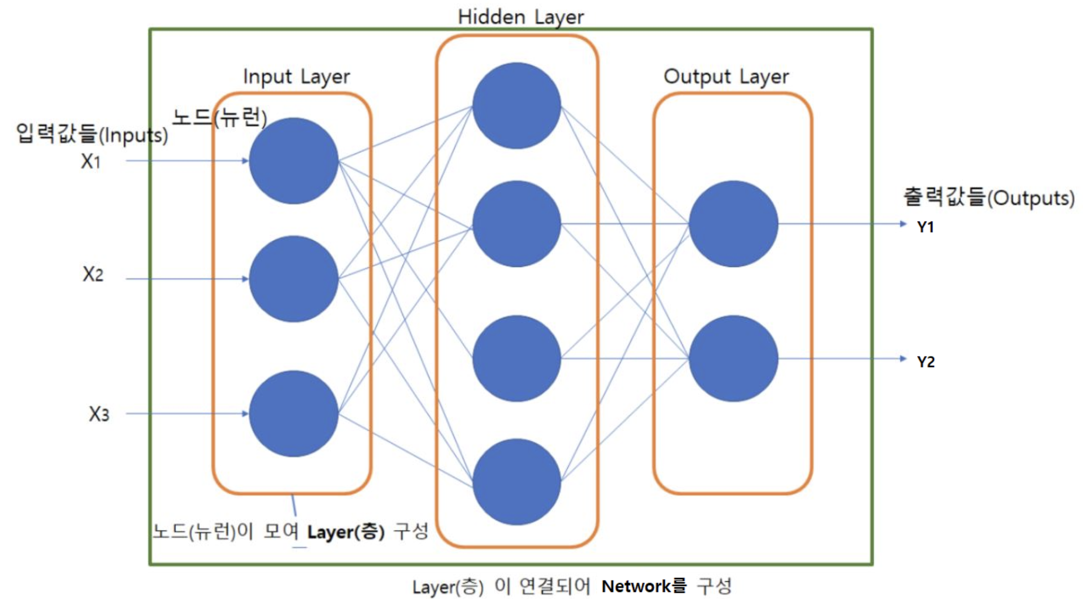
Universal Approximation Theorem이란 1개의 비선형 Activation함수를 포함하고 있는 히든 레이어를 가진 Neural Network를 이용해 어떠한 함수든 근사시킬 수 있다는 이론.

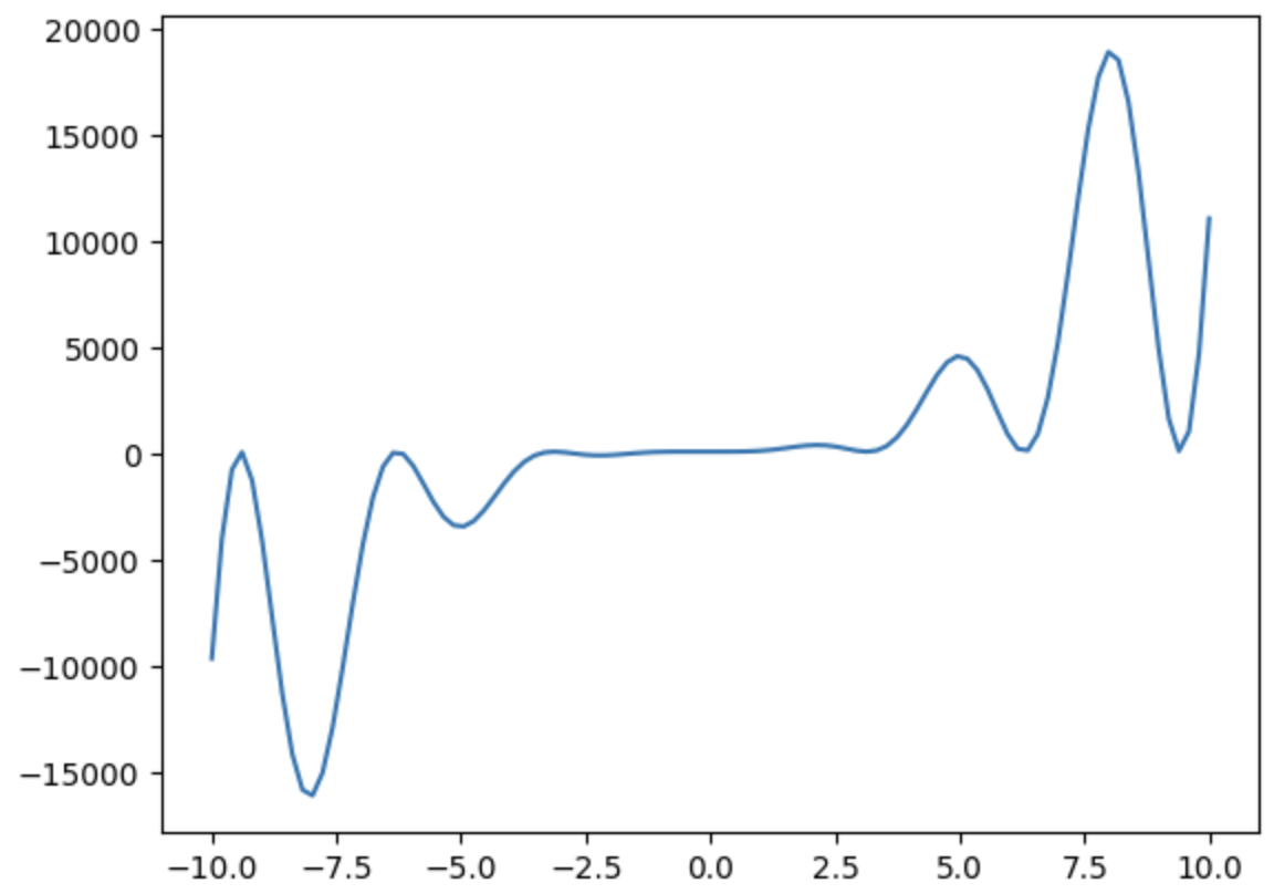
import numpy as np
import matplotlib.pyplot as plt
import torch
import torch.nn as nn
device = "cuda" if torch.cuda.is_available() else "cpu"

def func(x):
    """
    근사시키려는 함수
    """
    return 7*np.sin(x)*np.cos(x)*(2*x**2+5*x**3+x**2)*np.tan(x)+120 

x = np.linspace(-10, 10, 100)
y = func(x)

x

array([-10. , -9.7979798 , -9.5959596 , -9.39393939,
-9.19191919, -8.98989899, -8.78787879, -8.58585859,
-8.38383838, -8.18181818, -7.97979798, -7.77777778,
-7.57575758, -7.37373737, -7.17171717, -6.96969697,
-6.76767677, -6.56565657, -6.36363636, -6.16161616,
-5.95959596, -5.75757576, -5.55555556, -5.35353535,
-5.15151515, -4.94949495, -4.74747475, -4.54545455,
-4.34343434, -4.14141414, -3.93939394, -3.73737374,
-3.53535354, -3.33333333, -3.13131313, -2.92929293,
-2.72727273, -2.52525253, -2.32323232, -2.12121212,
-1.91919192, -1.71717172, -1.51515152, -1.31313131,
-1.11111111, -0.90909091, -0.70707071, -0.50505051,
-0.3030303 , -0.1010101 , 0.1010101 , 0.3030303 ,
0.50505051, 0.70707071, 0.90909091, 1.11111111,
1.31313131, 1.51515152, 1.71717172, 1.91919192,
2.12121212, 2.32323232, 2.52525253, 2.72727273,
2.92929293, 3.13131313, 3.33333333, 3.53535354,
3.73737374, 3.93939394, 4.14141414, 4.34343434,
4.54545455, 4.74747475, 4.94949495, 5.15151515,
5.35353535, 5.55555556, 5.75757576, 5.95959596,
6.16161616, 6.36363636, 6.56565657, 6.76767677,
6.96969697, 7.17171717, 7.37373737, 7.57575758,
7.77777778, 7.97979798, 8.18181818, 8.38383838,
8.58585859, 8.78787879, 8.98989899, 9.19191919,
9.39393939, 9.5959596 , 9.7979798 , 10. ])

y

array([-9.61705008e+03, -3.98831643e+03, -7.21318592e+02, 9.41775339e+01,
-1.23298184e+03, -4.09229365e+03, -7.70728865e+03, -1.12827929e+04,
-1.41376494e+04, -1.58022191e+04, -1.60683775e+04, -1.49893127e+04,
-1.28353912e+04, -1.00191958e+04, -7.00657752e+03, -4.23088831e+03,
-2.02481714e+03, -5.79277382e+02, 6.72403804e+01, 1.13162728e+01,
-5.53613164e+02, -1.38643734e+03, -2.24805212e+03, -2.94250151e+03,
-3.34345618e+03, -3.40355195e+03, -3.14770160e+03, -2.65434563e+03,
-2.03027132e+03, -1.38494559e+03, -8.09405447e+02, -3.62985074e+02,
-6.90151843e+01, 8.13972792e+01, 1.19908210e+02, 8.89413862e+01,
3.02517980e+01, -2.35820235e+01, -5.34898569e+01, -5.40276488e+01,
-3.02436574e+01, 7.15640230e+00, 4.66959860e+01, 7.97565044e+01,
1.02262163e+02, 1.14435029e+02, 1.19209378e+02, 1.20198452e+02,
1.20084994e+02, 1.20001812e+02, 1.20002546e+02, 1.20258452e+02,
1.22309640e+02, 1.29651561e+02, 1.47170150e+02, 1.79383195e+02,
2.27962012e+02, 2.89424509e+02, 3.54053538e+02, 4.06912467e+02,
4.31308424e+02, 4.14302254e+02, 3.53075961e+02, 2.60375393e+02,
1.67059322e+02, 1.20135305e+02, 1.75550257e+02, 3.86286361e+02,
7.87719868e+02, 1.38338417e+03, 2.13489292e+03, 2.95956498e+03,
3.73815582e+03, 4.33315447e+03, 4.61567915e+03, 4.49659110e+03,
3.95561069e+03, 3.06148179e+03, 1.97693628e+03, 9.44433450e+02,
2.52133830e+02, 1.83744272e+02, 9.59937986e+02, 2.68211861e+03,
5.29056089e+03, 8.54789539e+03, 1.20554029e+04, 1.53040336e+04,
1.77553278e+04, 1.89407060e+04, 1.85622825e+04, 1.65756883e+04,
1.32362406e+04, 9.09444124e+03, 4.93477437e+03, 1.66194756e+03,
1.49346138e+02, 1.07354479e+03, 4.76430149e+03, 1.11000778e+04])

plt.plot(x, y)
plt.show()

# x, y를 tensor
X_train = torch.tensor(x, dtype=torch.float32).unsqueeze(1).to(device)
y_train = torch.tensor(y, dtype=torch.float32).unsqueeze(1).to(device)
X_train.shape, y_train.shape

(torch.Size([100, 1]), torch.Size([100, 1]))

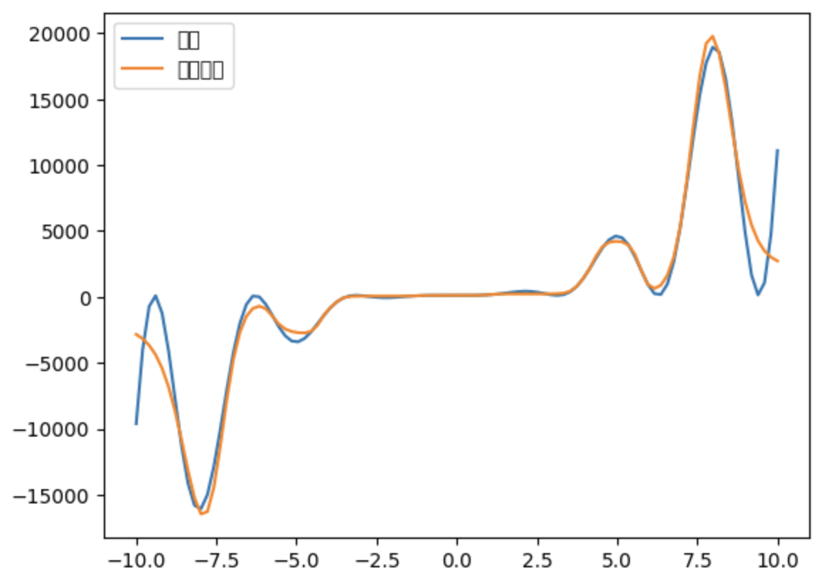
# input -> Linear -> activation함수 -> Linear -> output
activation_fn = nn.Tanh() # hyperbolic tangent
model = nn.Sequential(
	nn.Linear(1, 10000),
    activation_fn,
    nn.Linear(10000, 1)
)
### 학습
model.to(device)
loss_fn = nn.MSELoss()
optim = torch.optim.RMSprop(model.parameters(), lr=0.01)
model.train()
for epoch in range(5000) :
	pred = model(X_train)
    loss = loss_fn(pred, y_train)
    loss.backward()
    optim.step()
    optim.zero_grad()

y_hat = model(X_train)
y_hat_arr = y_hat.to("cpu").detach().numpy().flatten()
plt.plot(x, y, label="정답")
plt.plot(x, y_hat_arr, label="모델추정")
plt.legend()
plt.show()