Sin Curve
numpy.sin()에 x값을 인자로 넘겨주면 해당하는 y 값들을 리턴한다.
X = numpy.linspace(0, 2 * numpy.pi, 100)
Y = numpy.sin(X)

plot.plot(X, Y)
plot.show()
Dotted Curve
X = numpy.linspace(-3, 2, 30) # -3에서 2까지 구간의 개수는 100개
Y = X ** 2 - 2 * X + 1.
Z = X ** 3 - 10 * X - 5

plot.plot(X, Y, '.b-')
plot.plot(X, Z, 'xr')  # 점은 x로 마킹하고 이어 주는 작업은 없다.
plot.legend(["Tomato", "Apple"])
plot.show()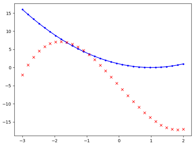
Read from Text
import matplotlib.pyplot as plot

X, Y, Z = list(zip(*[[float(s) for s in line.split()] for line in open('sample.txt', 'r')])) # 파일에서 읽어오기

plot.plot(X, Y)
plot.show()
data = numpy.loadtxt('sample.txt')
plot.plot(data[:,0], data[:,1])
plot.show()Sub Plot
from matplotlib.pyplot import *

x = [1,2,3,4]
y = [5,4,3,2]

figure()

subplot(231)
plot(x, y)

subplot(232)
bar(x, y)

subplot(233)
barh(x, y)

subplot(234)
bar(x, y)
y1 = [7,8,5,3]
bar(x, y1, bottom=y, color = 'r')

subplot(235)
boxplot(x)

subplot(236)
scatter(x,y)

show()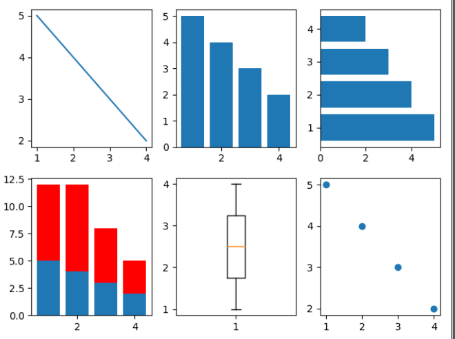
sub plots two functions
subplot의 개수는 add_subplot 메서드의 인자를 통해 조정할 수 있다. 다음 코드에서 (2, 1, 1)은 2x1(행x열)의 subplot을 생성한다는 의미이고 세 번째 인자 1은 생성된 두 개의 subplot 중 첫 번째 subplot을 의미한다. 마찬가지로 (2, 1, 2)는 2x1 subplot에서 두 번째 subplot을 의미한다.
import numpy as np
import matplotlib.pyplot as plt

x = np.arange(0.0, 2 * np.pi, 0.1)
sin_y = np.sin(x)
cos_y = np.cos(x)

fig = plt.figure()
ax1 = fig.add_subplot(2, 1, 1)
ax2 = fig.add_subplot(2, 1, 2)

ax1.plot(x, sin_y, 'b--')
ax2.plot(x, cos_y, 'r--')

plt.show()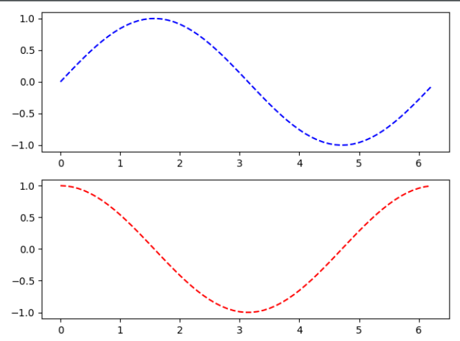
Grid SubPlot
import matplotlib.pyplot as plt
import numpy as np
plt.style.use('seaborn-white')

for i in range(1, 7):
    plt.subplot(2, 3, i)
    plt.text(0.5, 0.5, str((2, 3, i)),
             fontsize=18, ha='center')

plt.show()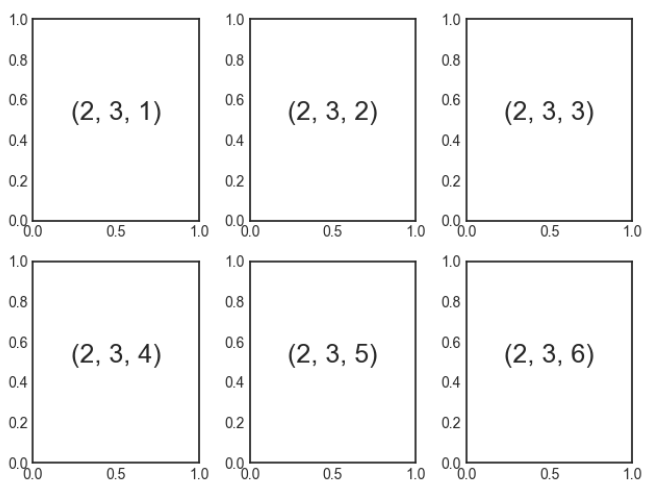

어려운 문제를 함께 풀어가는 것을 좋아합니다.