[Vision Transformer] An Image is Worth 16x16 Words: Transformers for Image Recognition at Scale 논문 리뷰

투빅스 14기 김민경
paper : An Image is Worth 16x16 Words: Transformers for Image Recognition at Scale (ViT)

1. INTRODUCTION

• 자연어 처리(NLP)에서는 Self-attention 기반 아키텍처, 특히 Transformer를 주로 사용한다.
• Transformer의 계산 효율성과 scalability 덕분에, 100B 이상의 파라미터를 사용하여 전례없는 크기의 모델을 학습할 수 있게 되었다.
• 그러나, 컴퓨터비전에서는 CNN 아키텍처가 여전히 우세하다.
• NLP 성공에 영감을 받은 여러 연구는 CNN과 유사한 아키텍처를 self-attention과 결합하려고 시도했지만, 대규모 이미지 인식에서 고전적인 ResNet같은 아키텍처가 여전히 SOTA이다.

• 해당 논문에서는 NLP의 Transformer 확장 성공에 영감을 받아, 가능한 최소한의 수정으로 standard Transformer를 이미지에 직접 적용하는 실험을 한다.
• strong regularization 없이 ImageNet과 같은 Mid-sized datasets에 대해 train된 경우, 비슷한 크기의 ResNet보다 몇 % 낮은 정확도를 보여준다.
  → 이는 겉보기에 실망스러운 결과일 수 있다.
  → Transformers는 CNN 고유의 Translation Invariance과 Locality 같은 Inductive Biases가 부족해서 충분하지 않은 양의 데이터로 train할 때 잘 일반화되지 않기 때문이다.

• Inductive Bias?
  : 학습 시에는 경험하지 않은 input이 주어져도 output의 적절한 귀납적 추론이 가능하도록 하기 위한 일련의 가정
• 문제(데이터)의 특성에 맞게 적절한 Inductive Bias를 가지는 알고리즘을 사용해야 높은 성능을 낼 수 있는데,
  CNN은 Locality와 Transitional Invariance한 특성을
  RNN은 Sequentiality와 Temporal Invariance한 특성을 가진다.

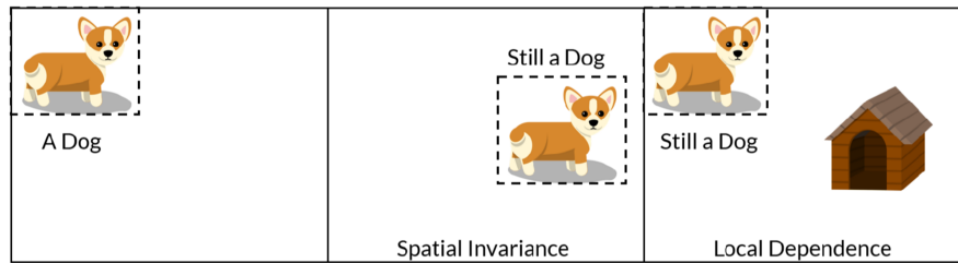
• Local Translation Invariance
  : 이미지의 모양이나 위치가 변하더라도 이미지에서 객체를 인식할 수 있다.
  

출처 : https://medium.com/analytics-vidhya/cnn-convolutional-neural-network
-8d0a292b4498

• 그러나 모델이 더 큰 datasets(14M-300M images)에서 train되면 결과가 달라진다.
• 즉, 대규모 training이 inductive bias를 능가한다는 것을 알 수 있다.
• Vision Transformer(ViT)는 충분한 규모로 pre-train 되어 더 적은 datapoints를 사용하는 태스크로 transfer될 때 탁월한 결과를 얻을 수 있다.
• public ImageNet-21k dataset 또는 사내 JFT-300M dataset에 대해 pre-train 된 ViT는 여러 이미지 인식 벤치마크에서 SOTA에 접근하거나 능가한다.
• 특히 best 모델은
  ImageNet에서 88.55%,
  ImageNet-ReaL에서 90.72%,
  CIFAR-100에서 94.55%,
  19개 태스크가 있는 VTAB 모음에서 77.63%의 정확도를 달성한다.

2. Method

2.1 Vision Transformer (ViT)

• 모델 디자인은 가능한 한 original Transformer (encoder 부분만 사용)를 따른다.
• Embedding Layer, Encoder, Final Head Classifier로 구성된다.
• Transformer encoder 부분과의 차이점은 이미지를 네트워크에 공급하는 방법에 있다.

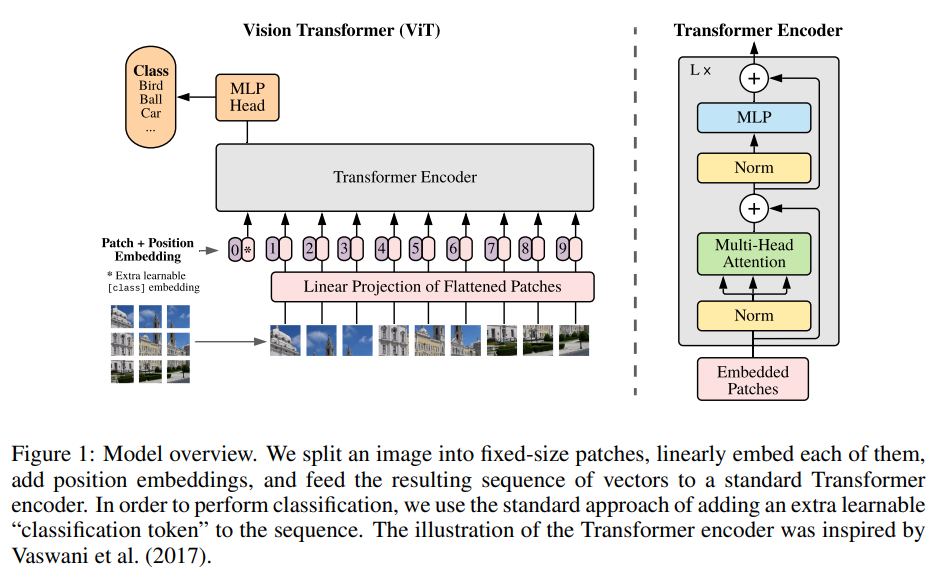
• ViT 네트워크 과정의 순서는 다음과 같다.
  1. 이미지를 patches로 분할 후 flatten
  2. flattened patches에서 저차원 linear embeddings 생성
  3. Position embeddings 추가
  4. 시퀀스를 Standard Transformer encoder에 input으로 공급
  5. 이미지 labels로 모델 pre-train
  (대용량 dataset에서 fully supervised)
  6. 이미지 classification를 위한 downstream dataset에 대해 fine-tuning

---

1. 이미지를 patches로 분할 후 flatten

• standard Transformer의 input은 token embeddings의 1D 시퀀스이다.
• 따라서 2D 이미지를 처리하기 위해 이미지 $\mathbf{x} ∈ \mathbb{R}^{H × W × C}$를
  일련의 flattened 2D 패치 $\mathbf{x}_p ∈ \mathbb{R}^{N × (P^2 · C)}$로 reshape한다.
  • 여기서 $(H, W)$는 원본 이미지의 해상도,
    $C$는 채널 수,
    $(P, P)$는 각 이미지 패치의 resolution이고,
    $N = HW / P^2$는 얻게되는 patches 수이며, input 시퀀스 길이로 간주
• 일반적으로 patch 사이즈 $P$는 16×16 또는 32×32로 선택되며, patch 사이즈가 작을수록 시퀀스가 길어진다. (→ 모델의 전체 정확도가 향상)
• 여기서 논문의 제목인 "An Image is Worth 16X16 Words"가 나왔다.

---

2. flattened patches에서 저차원 Linear embeddings 생성

• Transformer는 모든 레이어를 통해 일정한 latent vector size $D$를 사용하므로 patches를 flatten하게 하고,
  trainable Linear Projection(아래 식)을 사용하여 $D$차원에 매핑한다.
  
• $E$는 learned embedding matrix를 의미
• 이 Linear Projection의 output을 Patch embeddings라고 한다.

---

3. Position embeddings 추가

• Position embeddings는 위치 정보를 유지하기 위해 Patch embeddings에 추가된다.
  
• $\mathbb{R}^{N × D}$이 아닌 $\mathbb{R}^{(N+1) × D}$인 이유?
  : embedded patches의 시퀀스 맨 앞에 [class] token ($\mathbf{x}_{class}$=$\mathbf{z}_0^0$)을 concat하기 때문 (BERT와 동일)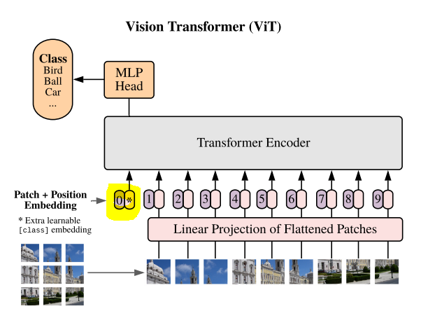
• 실험에서 1-D positional encodings과 2-D positional encodings이 거의 동일한 결과를 생성하는 것으로 나타났기 때문에 단순한 standard learnable 1D position embeddings를 사용하여 flattened patches의 위치 정보를 보존한다.
• 결과 embedding vetors의 시퀀스($\mathbf{z}_0$)는 $L$개의 동일한 레이어로 구성된 Transformer encoder의 input이 된다.

---

4. 시퀀스를 Standard Transformer encoder에 input으로 공급

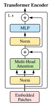
• Transformer encoder는 Multihead Self-Attention(MSA)과 MLP blocks로 구성된다.
• LayerNorm(LN)은 모든 블록 이전에 적용되고 Residual Connections는 모든 블록 이후에 적용된다.
• MLP는 GELU non-linearity가 있는 두 개의 레이어로 구성된다.
  
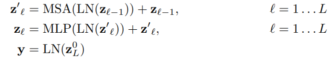
• Transformer encoder의 ouput에서 시퀀스의 첫 번째 요소인 $\mathbf{z}_L^0$을 MLP Head(Classification head)에 넣어 class label을 예측 한다.

# ViT 구현
# 출처 : https://theaisummer.com/vision-transformer/

import torch
import torch.nn as nn
from einops import rearrange
from self_attention_cv import TransformerEncoder

class ViT(nn.Module):
    def __init__(self, *,
                 img_dim,
                 in_channels=3,
                 patch_dim=16,
                 num_classes=10,
                 dim=512,
                 blocks=6,
                 heads=4,
                 dim_linear_block=1024,
                 dim_head=None,
                 dropout=0, transformer=None, classification=True):
        """
        Args:
            img_dim: the spatial image size
            in_channels: number of img channels
            patch_dim: desired patch dim
            num_classes: classification task classes
            dim: the linear layer's dim to project the patches for MHSA
            blocks: number of transformer blocks
            heads: number of heads
            dim_linear_block: inner dim of the transformer linear block
            dim_head: dim head in case you want to define it. defaults to dim/heads
            dropout: for pos emb and transformer
            transformer: in case you want to provide another transformer implementation
            classification: creates an extra CLS token
        """
        super().__init__()
        assert img_dim % patch_dim == 0, f'patch size {patch_dim} not divisible'
        self.p = patch_dim
        self.classification = classification
        tokens = (img_dim // patch_dim) ** 2
        self.token_dim = in_channels * (patch_dim ** 2)
        self.dim = dim
        self.dim_head = (int(dim / heads)) if dim_head is None else dim_head
        self.project_patches = nn.Linear(self.token_dim, dim)
        self.emb_dropout = nn.Dropout(dropout)
        
        if self.classification:
            self.cls_token = nn.Parameter(torch.randn(1, 1, dim))
            self.pos_emb1D = nn.Parameter(torch.randn(tokens + 1, dim))
            self.mlp_head = nn.Linear(dim, num_classes)
        else:
            self.pos_emb1D = nn.Parameter(torch.randn(tokens, dim))
        
        if transformer is None:
            self.transformer = TransformerEncoder(dim, blocks=blocks, heads=heads,
                                                  dim_head=self.dim_head,
                                                  dim_linear_block=dim_linear_block,
                                                  dropout=dropout)
        else:
            self.transformer = transformer
    
    def expand_cls_to_batch(self, batch):
        """
        Args:
            batch: batch size
        Returns: cls token expanded to the batch size
        """
        return self.cls_token.expand([batch, -1, -1])
    
    def forward(self, img, mask=None):
        batch_size = img.shape[0]
        # 이미지를 patches로 분할 후 flatten
        img_patches = rearrange(
            img, 'b c (patch_x x) (patch_y y) -> b (x y) (patch_x patch_y c)',
                                patch_x=self.p, patch_y=self.p)
        
        # Linear Projection
        img_patches = self.project_patches(img_patches)
        if self.classification:
            img_patches = torch.cat(
                (self.expand_cls_to_batch(batch_size), img_patches), dim=1)
        
        # Position embeddings 추가
        patch_embeddings = self.emb_dropout(img_patches + self.pos_emb1D)
        
        # feed patch_embeddings and output of transformer. shape: [batch, tokens, dim]
        y = self.transformer(patch_embeddings, mask)
        
        if self.classification:
            # we index only the cls token for classification. 
            return self.mlp_head(y[:, 0, :])
        else:
            return y

2.2 Pre-training & Fine-tuning

5. Pre-training

• 1k개 클래스, 1.3M개의 이미지가 있는 ImageNet,
  21k개 클래스, 14M개의 이미지가 있는 superset ImageNet-21k,
  18k개 클래스, 303M개의 고해상도 이미지가 있는 Google private JFT를 사용

• weight decay = 0.1, batch size = 4096, $β_1$ = 0.9, $β_2$ = 0.999인 Adam optimizer를 사용한다.

6. Fine-tuning

• Pre-training 에 사용된 입력 이미지보다 높은 해상도로 Fine-tuning을 수행한다.
• train된 모델들을 여러 벤치마크 tasks로 transfer한다.
  : original ImageNet, ImageNet-ReaL, CIFAR-10/100, Oxford-IIIT Pets와 Oxford Flowers-102, VTAB(Natural, Specialized, Structured)
• 모든 모델에 대해 batch size = 512인 SGD w/ momentum을 사용한다.

---

* Hybrid Architecture (ViT의 변형)

• input 시퀀스인 raw image patches는 CNN의 피처맵으로 대체될 수 있다.
• Hybrid model은 patch embedding projection $E$가 CNN 피처맵에서 추출된 patch들에 적용된다.

• 해당 논문에서는 실험을 위해 ViT에 ResNet50을 이미지에 적용하여 얻은 intermediate 피처맵을 input으로 주었다. (patch 사이즈가 "pixel"임)
• 아래 그림은 ViT, Hybrid, ResNets 세 모델의 pre-training compute 성능을 나타낸 것이다.
  

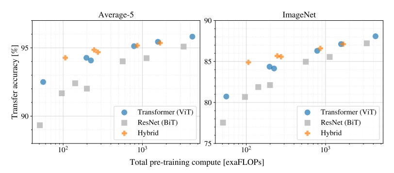
• ViT는 동일한 computational budget으로 ResNet을 능가한다.
  (ViT는 동일한 성능을 얻기 위해 약 2~4배 적은 컴퓨팅을 사용)
• Hybrid는 모델 크기가 작은 경우 기본 ViT보다 향상되고 모델 크기가 커지면서 차이가 사라지는 것을 볼 수 있다.
  → 어떤 사이즈에서든 ViT를 지원하는 컨볼루션 local feature processing을 기대할 수 있기 때문에 향후 주목할만 하다.
• 또한, ViT는 실험된 범위 내에서 "saturate"되지 않는 것으로 보이기 때문에 향후 확장 가능성을 기대할만 하다.

3. Experiments

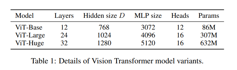
3.1 Vision Transformer Variants

• classification 정확도에 대한 모델 사이즈 증가의 효과를 실험하기 위해
  "ViT-Base", "ViT-Large", "ViT-Huge"와 같은 다양한 버전의 ViT를 제안한다.
• 세 가지 버전은 encoder의 레이어 수, hidden dimension 사이즈, MSA 레이어에서 사용하는 attention head 수, MLP classifier 사이즈가 다르다.
  
• 각 모델은 16×16, 32×32 크기의 patch로 학습된다.
• ViT-Base
  : Transformer encoder에 12개의 레이어, 12개의 attention heads, 768의 hidden dimension 사이즈를 가진다.
• ViT-Large
  : Transformer encoder에 24개의 레이어, 16개의 attention heads, 1024의 hidden dimension 사이즈를 가진다.
• ViT-Huge
  : Transformer encoder에 32개의 레이어, 16 개의 attention heads, 1280의 hidden dimension 사이즈를 가진다.

• 다른 크기를 갖는 Vision Transformers에 대한 실험 결과는
  더 높은 정확도를 얻기 위해 상대적으로 더 깊은 모델을 사용하는 것이 중요하다는 것을 보여준다.

3.2 Comparison to State Of The Art

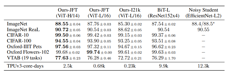
• JFT-300M에서 pre-training된 더 작은 ViT-L/16 모델은 모든 태스크에서 BiT-L(동일한 dataset에 대해 pre-training 됨)보다 성능이 뛰어나며 학습에 필요한 컴퓨팅 리소스가 훨씬 적다.
• 더 큰 모델인 ViT-H/14는 특히 ImageNet, CIFAR-100와 VTAB과 같은 보다 까다로운 datasets에서 성능을 더욱 향상시킨다.
• 이 모델은 이전의 SOTA보다 pre-training에 훨씬 적은 컴퓨팅을 사용했다.

• 아래 표는 VTAB를 Natural, Specialized, Structured 각 그룹으로 분해하고, 이 벤치마크에서 이전 SOTA 방법과 비교한 결과이다.
  
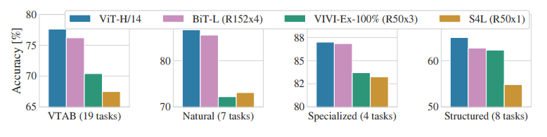
• ViT-H/14는 Natural과 Structured 태스크에서 BiT-L(152x4)과 기타 방법들을 능가한다.

3.2 Inspecting Vision Transformer

• ViT가 이미지를 처리하는 과정을 이해하기 위해 내부 표현을 분석하는 실험을 했다.

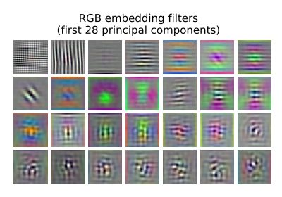
(1) Filters of the initial linear embedding of RGB values of ViT-L/32

• Vision Transformer의 첫 번째 레이어는 flattened patches를 더 낮은 차원의 공간에 Linearly Projection한다.
• 아래 그림은 학습된 embedding filters의 주성분(principal components)을 보여준다.
  

(2) Similarity of position embeddings of ViT-L/32

• 아래 그림은 모델이 position embeddings의 similarity에서 이미지 내 거리를 인코딩하는 방법을 학습함을 보여준다.
  즉, 더 가까운 patches는 더 유사한 position embeddings를 갖는 경향이 있다.
• 또한 row-column structure가 나타난다.
  : 동일한 행/열에 있는 patches는 유사한 embeddings을 가진다.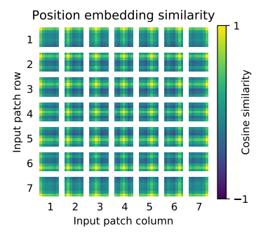

(3) Size of attended area by head and network depth

• Self-attention을 통해 ViT는 가장 낮은 레이어에서도 전체 이미지에 대한 정보를 통합할 수 있게한다.
• 아래 그림은 네트워크가 이 기능을 어느 정도 사용하는지 알아본 실험 결과이다.
  (head와 network depth에 따른 attended area의 사이즈)
• 각 점은 한 레이어에있는 16개의 head 중 하나에 대한 이미지에서의 attention distance를 의미한다.
  
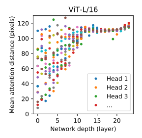
• 일부 heads가 이미 가장 낮은 레이어에 있는 대부분의 이미지에 주의를 기울여 정보를 global하게 통합하는 기능이 실제로 모델에서 사용됨을 알 수 있다.
  반면, 다른 attention heads는 낮은 레이어에서 지속적으로 작은 attention distances를 갖는다.

4. Conclusion

• Image Recognition에 Transformers를 직접 적용하는 방법을 살펴 보았다.
• 컴퓨터비전에서 self-attention을 사용하는 이전 연구들과 달리, 해당 연구는 초기 patch extraction 단계를 분리하여 image-specific inductive biases를 아키텍처에 도입하지 않는다.
  대신 이미지를 patches 시퀀스로 해석하고 NLP에서 사용되는 standard Transformer encoder로 처리한다.
• 이 간단하면서도 확장 가능한 전략은 대규모 datasets에 대한 pre-training과 결합될 때 매우 잘 작동한다.
• 따라서 Vision Transformer는 많은 image classification datasets에서 SOTA 비슷하거나 능가하는 동시에 pre-training 비용이 상대적으로 낮다.
• 이러한 초기 결과는 고무적이지만 많은 과제가 남아 있다.
  (1) detection과 segmentation 같은 다른 컴퓨터비전 태스크에 ViT를 적용하는 것
  (2) self-supervised pre-training 방법을 계속 탐구하는 것
• 우리의 초기 실험은 self-supervised pre-training의 개선을 보여주지만, self-supervised pre-training과 large-scale supervised pre-training 사이에는 여전히 큰 차이가 있다.
• 마지막으로 ViT를 추가로 확장하면 성능이 향상될 수 있다.

---

5. 질문 내용 추가

(1) Attention Distance

Q. "attention distance"의 개념이 궁금합니다.
A. CNN의 receptive field size와 유사한 개념이라고 합니다.

→ 참고 https://www.analyticsvidhya.com/blog/2021/03/an-image-is-worth-16x16-words-transformers-for-image-recognition-at-scale-vision-transformers/

(2) Self-supervised

Q. ViT에서 Self-supervised가 어떻게 학습이 되나요?
A. 논문의 APPENDIX B.1.2에서 masked patch prediction objective를
이용했다고 합니다.
그러나 간략하게만 설명해 놓았기 때문에 추가 자료를 덧붙이겠습니다.
Self-supervised vision Transformer를 제안한 논문인 SiT: Self-supervised vIsion Transformer를 참고하시면 좋을 것 같습니다:)

• 이 연구의 주요 목표는 unsupervised 방식으로 data representation을 학습하는 것이다.
• 이것은 이미지의 일부가 masking되거나 transform된 local 부분을 완성함으로써 달성된다.
• 기본 가설은 전체 visual field의 context를 기반으로 이미지의 손상된 부분을 손상되지 않은 부분에서 복구함으로써 네트워크가 visual integrity(무결성)의 개념을 은연중에 학습한다는 것이다.
  
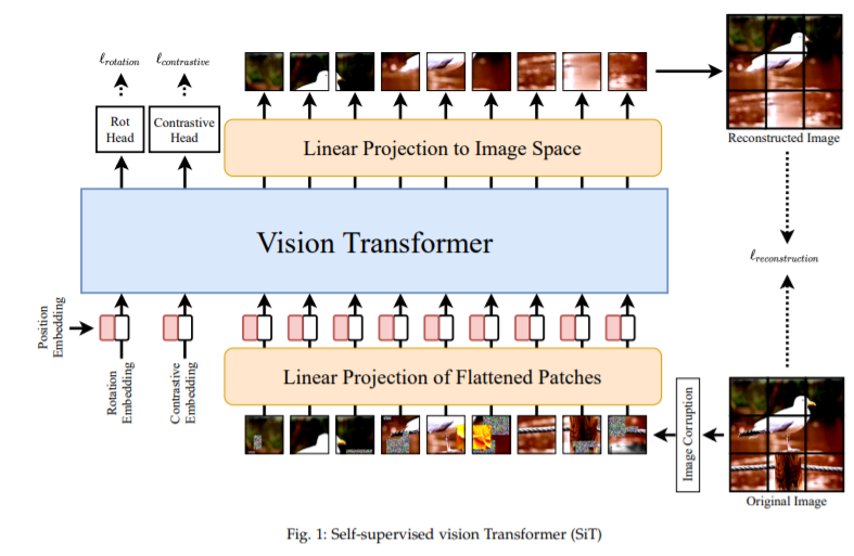
• (1) Image reconstruction, (2) Rotation prediction, (3) Contrastive learning 이렇게 세 개의 objectives를 사용해서 train한다.

(3) ViT에서 Q, K, V의 의미

• 아래 링크들을 참고하시면 좋을 것 같습니다.
• https://www.youtube.com/watch?v=QkwNdgXcfkg&t=348s&ab_channel=%ED%85%90%EC%B4%88
  13:00 부터 참고
• https://hongl.tistory.com/234

---

REFERENCE

• https://enfow.github.io/paper-review/graph-neural-network/2021/01/11/relational_inductive_biases_deep_learning_and_graph_netowrks/
• https://keras.io/examples/vision/image_classification_with_vision_transformer/
• https://theaisummer.com/vision-transformer/
• Vision Transformers for Remote Sensing Image Classification (Yakoub Bazi, Laila Bashmal, Mohamad M. Al Rahha, Reham Al Dayil and Naif Al Ajlan)
• https://engineer-mole.tistory.com/133