❕ 모든 장기가 포함된 CT 이미지 input으로 넣으면 모델 학습이 안 되기 때문에, 각 장기 별 모델 따로 구현
1. Data : patient id, series id, 장기별 healthy, low, high label encoding 값, bbox 좌표
- 이 중, bbox 값 negative인 row 제거
# Filter out rows where any of the bounding box coordinates are negative
filtered_df = df[~(df[['x_min', 'x_max', 'y_min', 'y_max', 'z_min', 'z_max']] < 0).any(axis=1)]- healthy patient 중 데이터에 중복되어 나타나는 경우 제외 ( healthy data가 너무 많아서 비율 맞추려는 것..? )
# Identify patient_ids with only 'kidney_healthy' labels
healthy_patient_ids = filtered_df[filtered_df['kidney_healthy'] == 1]['patient_id'].unique()
print(len(healthy_patient_ids))

# Filter out patient_ids that are duplicated
unique_healthy_patient_ids = filtered_df[~filtered_df['patient_id'].duplicated(keep=False) & filtered_df['patient_id'].isin(healthy_patient_ids)]
print(len(unique_healthy_patient_ids))

# Correctly concatenate the two dataframes using `pd.concat()`
filtered_df_reduced_by_patient_corrected = pd.concat([filtered_df[~filtered_df['patient_id'].isin(healthy_patient_ids)], unique_healthy_patient_ids])
2. healthy & injury 비율 맞추기
- 1:1, 2:1 비율로 시도 ; len(injury_df_new)에 맞춰 healthy sampling
- random seed = 42로 고정해 재현성 보장
- train, valid, test 모두 적용
# Create a new column 'kidney_injury' which is the sum of 'kidney_low' and 'kidney_high'
train_2['kidney_injury'] = train_2['kidney_low'] + train_2['kidney_high']

# Filter out the kidney_injury and kidney_healthy samples
injury_df_new= train_2[train_2['kidney_injury'] == 1]
healthy_df_new = train_2[train_2['kidney_healthy'] == 1]

# Randomly sample from kidney_healthy to match the count of kidney_injury (with a seed for reproducibility)
random_seed = 42
balanced_healthy_df_new = healthy_df_new.sample(n=len(injury_df_new), random_state=random_seed)

# Combine the datasets to achieve a 1:1 ratio
train = pd.concat([injury_df_new, balanced_healthy_df_new], ignore_index=True)

# Check the distribution in the new balanced dataset
train_distribution = train[['kidney_healthy', 'kidney_injury']].sum()
train_distribution
(❓injury에 맞춰 비율을 조절하면 데이터가 줄어드니, dc-gan으로 injury의 양을 늘리는건? 아무래도 fake img니까 결과를 신뢰하기가 어려울 수 있을 것 같음)
; https://www.kaggle.com/code/harshsingh2209/generating-brain-mri-images-with-dc-gan
3. pre-processing (train / val 동일하게 적용)
- 앞의 장기 별 3D bbox 좌표 추출
def extract_organ_3D_bounding_box(nii_file):
    """
    주어진 .nii 파일에서 장기의 3D bounding box (min, max 좌표)를 추출합니다.

    Args:
    - nii_file (str): .nii 파일의 경로.

    Returns:
    - dict: 장기 이름을 키로 하고 해당하는 min, max 3D 좌표를 값으로 가지는 딕셔너리.
    """

    # .nii 파일 불러오기
    nii_image = sitk.ReadImage(nii_file)
    data = sitk.GetArrayFromImage(nii_image)

    # 각 장기에 대한 bounding box 좌표를 저장할 사전
    organ_bounding_boxes = {}

    organ_labels = {
        'liver': [5],
        'spleen': [1],
        'kidney': [2, 3],
        'bowel': [55, 57, 56]  # small_bowel, colon, duodenum
    }

    # 각 장기의 bounding box 좌표 추출
    for organ, labels in organ_labels.items():
        coords = []
        for label in labels:
            coords.extend(np.argwhere(data == label).tolist())

        if not coords:
            organ_bounding_boxes[organ] = None
            continue

        coords = np.array(coords)

        z_min, y_min, x_min = coords.min(axis=0)
        z_max, y_max, x_max = coords.max(axis=0)

        # 각 차원의 중심을 계산
        z_center, y_center, x_center = (z_min + z_max) // 2, (y_min + y_max) // 2, (x_min + x_max) // 2

        # scale_factor 지정
        scale_factor = 1.2

        # 각 차원의 절반 길이를 계산
        z_half, y_half, x_half = (z_max - z_min) * scale_factor / 2, (y_max - y_min) * scale_factor / 2, (x_max - x_min) * scale_factor / 2

        # 중심을 기준으로 bounding box 재조정
        z_min, z_max = int(z_center - z_half), int(z_center + z_half)
        y_min, y_max = int(y_center - y_half), int(y_center + y_half)
        x_min, x_max = int(x_center - x_half), int(x_center + x_half)

        organ_bounding_boxes[organ] = {
            'x': (x_min, x_max),
            'y': (y_min, y_max),
            'z': (z_min, z_max)
        }

return organ_bounding_boxes- resampling w/ SimpleITK
ResampleImageFilter
; reference_image 설정 -> 참조 이미지의 크기, 픽셀 간격, 원점 등 속성 따르도록 함
Linear Interpolation
; resampling할 때 주변 픽셀(8개) weighted average 이용해 픽셀 값 재계산
def resample_to_reference(self,input_image, reference_image):
    """
    Resample the input_image to match the pixel spacing, size, and origin of the reference_image.
    """

    resampler = sitk.ResampleImageFilter()
    resampler.SetReferenceImage(reference_image)
    resampler.SetInterpolator(sitk.sitkLinear)

    resampled_image = resampler.Execute(input_image)
    return resampled_image
- 원하는 장기(kidney) roi 추출
- .nii 파일(Total Segmentator 결과)로 bbox 좌표 추출
- 이 .nii 파일 픽셀 간격, 크기, 원점 기준으로 DICOM 이미지 resampling
- resampling된 DICOM 이미지 numpy 배열로 변환
- bbox 이용해 3D image array 슬라이싱 해 roi 추출해 저장
- 이중에 관심 장기(kidney)만 organ_data 따로 저장
def extract_roi_from_dicom(self,patient_id,series_id):
        organ_data = {}
        series_folder = os.path.join(self.dicom_folder_path,patient_id, series_id)

        # .nii 파일 경로 생성
        nii_file = os.path.join(self.nii_folder_path , f"{patient_id}_{series_id}.nii")

        # Filter the DataFrame to get the ROI coordinates for the specific patient and series
        specific_roi = self.df[
            (self.df['patient_id'] == patient_id) &
            (self.df['series_id'] == series_id)
        ]
        organ_bounding_boxes = self.extract_organ_3D_bounding_box(nii_file)
        # if specific_roi.empty:

            # raise ValueError(f"No ROI coordinates found for patient_id {patient_id} and series_id {series_id}")

        x_min, x_max, y_min, y_max, z_min, z_max = specific_roi[['x_min', 'x_max', 'y_min', 'y_max', 'z_min', 'z_max']]

        # DICOM 파일들을 정렬된 순서로 로드
        dicom_series_reader = sitk.ImageSeriesReader()
        dicom_names = dicom_series_reader.GetGDCMSeriesFileNames(series_folder)
        dicom_series_reader.SetFileNames(dicom_names)
        dicom_3d_image = dicom_series_reader.Execute()

        # DICOM 이미지와 NIfTI 이미지의 방향 일치시키기
        nii_image = sitk.ReadImage(nii_file)

        # DICOM 이미지를 NIfTI 이미지의 픽셀 간격, 크기, 원점으로 재샘플링
        resampled_dicom_image = self.resample_to_reference(dicom_3d_image, nii_image)

        # 재샘플링된 DICOM 이미지를 standardize_pixel_array
        resampled_dicom_image = standardize_pixel_array_sitk(resampled_dicom_image)

        # 재샘플링된 DICOM 이미지를 배열로 변환
        dicom_array = sitk.GetArrayFromImage(resampled_dicom_image)

        # 각 장기의 ROI를 3D 배열로 추출
        organ_arrays = {}
        organ_arrays['dicom'] = dicom_array
        for organ, bbox in organ_bounding_boxes.items():
            x_min, x_max = bbox['x']
            y_min, y_max = bbox['y']
            z_min, z_max = bbox['z']
            organ_arrays[organ] = dicom_array[z_min:z_max+1, y_min:y_max+1, x_min:x_max+1]

        organ_data = organ_arrays['kidney']

return organ_data- pixel value standardize
- SimpleITK -> arry 변환
- meta 메이터 추출 + 비트 수 확인
- pixel 값 signed integer(음수 포함)이면 shifting으로 일단 양수로 표현(?)
- 픽셀 값 HU 단위로 변환 ( CT 이미지니까 )
- windowing 처리 w/ window center & width 설정
-> window 범위(관심 영역) 제외 어둡게 처리 - 픽셀 값 정규화 standardize(0-1) -> 이미지 대비 더욱 명확히
- 다시 np array -> SimpleITK 변환
def standardize_pixel_array_sitk(image: sitk.Image) -> sitk.Image:
    # SimpleITK 이미지에서 NumPy 배열로 픽셀 데이터를 가져옵니다.
    pixel_array = sitk.GetArrayFromImage(image)

    # 이미지의 메타데이터에서 필요한 정보를 가져옵니다.
    # PixelRepresentation: 픽셀이 어떻게 표현되는지 나타내며, 0은 unsigned integer, 1은 signed integer 입니다.
    pixel_representation = int(image.GetMetaData('0028|0103') if image.HasMetaDataKey('0028|0103') else '0')

    # BitsAllocated: 하나의 픽셀 값에 할당된 비트 수
    bits_allocated = int(image.GetMetaData('0028|0100') if image.HasMetaDataKey('0028|0100') else '16')

    # BitsStored: 실제 이미지 저장에 사용된 비트 수
    bits_stored = int(image.GetMetaData('0028|0101') if image.HasMetaDataKey('0028|0101') else '12')

    # PhotometricInterpretation: 이미지의 광학적 해석을 설명하는 데이터
    photometric_interpretation = image.GetMetaData('0028|0004') if image.HasMetaDataKey('0028|0004') else ''

    # PixelRepresentation 값이 1이면 픽셀 값의 범위를 조정합니다. (Signed integer 처리)
    if pixel_representation == 1:
        bit_shift = bits_allocated - bits_stored
        dtype = pixel_array.dtype
        pixel_array = (pixel_array << bit_shift).astype(dtype) >> bit_shift

    # PhotometricInterpretation이 "MONOCHROME1"이면 픽셀 값을 반전시킵니다.
    if photometric_interpretation == "MONOCHROME1":
        pixel_array = np.max(pixel_array) - pixel_array

    # 픽셀 값을 Hounsfield 단위로 변환합니다.
    # RescaleIntercept: 픽셀 값에 더해지는 값
    intercept = float(image.GetMetaData('0028|1052') if image.HasMetaDataKey('0028|1052') else '0')

    # RescaleSlope: 픽셀 값에 곱해지는 값
    slope = float(image.GetMetaData('0028|1053') if image.HasMetaDataKey('0028|1053') else '1')

    pixel_array = pixel_array * slope + intercept

    # Windowing 처리: 이미지의 대비를 조절합니다.
    window_center = int(float(image.GetMetaData('0028|1050')) if image.HasMetaDataKey('0028|1050') else 40)
    window_width = int(float(image.GetMetaData('0028|1051')) if image.HasMetaDataKey('0028|1051') else 400)

    img_min = window_center - window_width // 2
    img_max = window_center + window_width // 2

    pixel_array = pixel_array.copy()
    pixel_array[pixel_array < img_min] = img_min
    pixel_array[pixel_array > img_max] = img_max

    # 정규화: 픽셀 값을 0과 1 사이로 스케일링합니다.
    if pixel_array.max() == pixel_array.min():
        # 모든 픽셀 값이 동일한 경우, 영 이미지로 처리합니다.
        pixel_array = np.zeros_like(pixel_array)
    else:
        pixel_array = (pixel_array - pixel_array.min()) / (pixel_array.max() - pixel_array.min())

    # NumPy 배열을 다시 SimpleITK 이미지로 변환합니다.
    out_image = sitk.GetImageFromArray(pixel_array)

    # 원본 이미지로부터 메타데이터와 변환 정보를 복사합니다.
    out_image.CopyInformation(image)

    return out_image
- resize
; CNN input (256,256,256)으로 resize
4. Model : CNN
- architecture : ResNet10 W/ 4 layers
첫 번째 층- conv1 + bn1(batch normalization) + relu + Max Pooling
layer 1- conv1 + bn1 + relu + conv2 + bn2
layer 2~4- conv1 + bn1 + relu + conv2 + bn2 + downsampling(conv + bn)
Avg Pooling[feature map (1,1,1)로 줄임(압축)] + FC layter[feature 512]
+) batch normalization ; 데이터 분포 정규화 -> 학습 안정화 & 과적합 방지
down sampling ; 입출력 차원 맞춰 주기 위함
- metrics ( binary / multi )
; binary [healthy / injury] - sigmoid
multi [healthy / low / high] - softmax
- hyper param
epoch: 100
batch: 2
optim: Adam
loss: BCEWithLogitsLoss (binary) / CrossEntropyLoss (multi)
scheduler: ReduceLROnPlateau (patience : 5 이후 factor : 0.5로 lr 줄임)
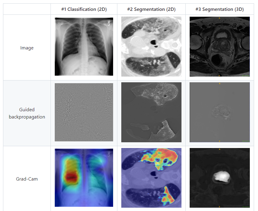
5. test 시 Med Cam / Grad Cam 적용
- Grad Cam
; CNN 모델이 어느 곳을 보고 있는지를 알려주는 weak supervised learning 알고리즘
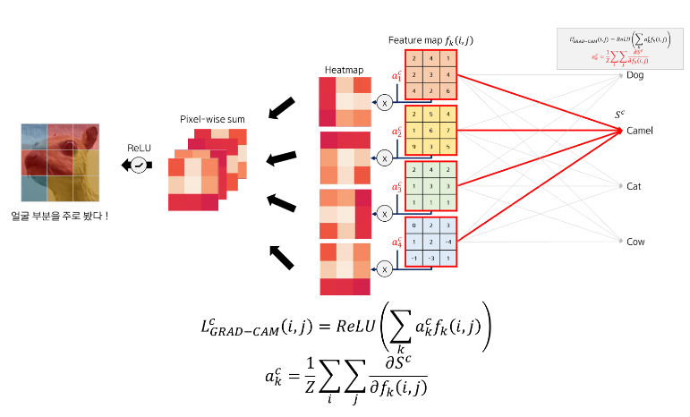
1. Gradient의 픽셀별 평균값(a)을 각 feature map(f)에 곱해 heatmap 생성
2. feature map 개수만큼 생성된 heat map을 pixel-wise sum함
3. Grad-CAM 결과 (attention map)
참고 - https://tyami.github.io/deep%20learning/CNN-visualization-Grad-CAM
- Med Cam ( https://github.com/MECLabTUDA/M3d-Cam )
; Grad Cam 기반 +3D에도 적용 가능
- acc & AUC 확인
# DataLoader 설정: 배치 크기를 1로 설정
test_loader = DataLoader(Valid_spleenDataset(test), batch_size=1, shuffle=True)

# 기존 모델 로드 및 설정
loaded_model = torch.load('/data/workspace/choie1/kaggle/rsna/input/prepro_data_4/model/spleen_1212/spleen_best_model_10.pth')
loaded_model.eval()

# Medcam 적용
from medcam import medcam

# label=1로 설정
loaded_model = medcam.inject(loaded_model, output_dir="/data/workspace/choie1/kaggle/rsna/input/prepro_data_4/spleen_map/",
                             backend='gcam', layer='module.backbone.layer4', label=0, save_maps=False, return_attention=True)

# Lists to store true and predicted labels
series_ids = []

# Initialize metrics
test_acc_spleen = MetricsCalculator('binary')

# Evaluation loop
with torch.no_grad():
    for batch_idx, batch_data in enumerate(test_loader):
        inputs = batch_data['image'].to(device)
        spleen = batch_data['spleen'].to(device).float()

        # Store series_id
        series_id = batch_data['series_id'][0]  # Assuming series_id is a list
        series_ids.extend(batch_data['series_id'])

        # Get prediction and attention map
        try:
            prediction, attention_map = loaded_model(inputs)
            test_acc_spleen.update(prediction, spleen)

            # Save the resized attention_map here
            attention_map_large = attention_map.squeeze().cpu().numpy()  # Remove singleton dimensions and convert to NumPy
            attention_map_large_sitk = sitk.GetImageFromArray(attention_map_large)  # Convert to SimpleITK Image

            new_file_name = f"/data/workspace/choie1/kaggle/rsna/input/prepro_data_4/spleen_map/module.backbone.layer4/attention_map_{series_id}.nii.gz"
            sitk.WriteImage(attention_map_large_sitk, new_file_name)

        except ValueError as ve:
            print(f"Error: {ve}")
            continue


# Print the results
print(f"Test Accuracy for spleen: {test_acc_spleen.compute_accuracy():.3f}")
print(f"Test AUC for spleen: {test_acc_spleen.compute_auc():.3f}")

# Plotting the confusion matrix
cm = confusion_matrix(test_acc_spleen.targets, test_acc_spleen.predictions)
plt.figure(figsize=(10, 8))
sns.heatmap(cm, annot=True, fmt='g', cmap='Blues')
plt.xlabel('Predicted labels')
plt.ylabel('True labels')
plt.title('Confusion Matrix')
plt.show()


# Create a DataFrame to store series_id, true labels, and predicted labels
results_df = pd.DataFrame({
    'series_id': series_ids,
    'True_Labels': test_acc_spleen.targets,
    'Predicted_Labels': test_acc_spleen.predictions
})

# Save the DataFrame to a CSV file
results_df.to_csv('/data/workspace/choie1/kaggle/rsna/input/prepro_data_4/spleen_predictions.csv', index=False)
6. 결과 확인 ( confusion metrics / image direction / 3D volume value 확인)
- 원본 이미지에 attention map(아마 medcam 결과) overlay해 시각화
      def display_overlay(volume, attention_map):
          def plot_slice(slice_idx):
              plt.figure(figsize=(12, 6))

        plt.subplot(1, 3, 1)
        plt.imshow(volume[slice_idx, :, :], cmap='gray')
        plt.title(f'Slice {slice_idx} - Original')
        plt.axis('off')

        plt.subplot(1, 3, 2)
        plt.imshow(attention_map[slice_idx, :, :], cmap='jet')
        plt.title(f'Slice {slice_idx} - Attention Map')
        plt.axis('off')

        plt.subplot(1, 3, 3)
        plt.imshow(volume[slice_idx, :, :], cmap='gray')
        plt.imshow(attention_map[slice_idx, :, :], alpha=0.5, cmap='jet')
        plt.title(f'Slice {slice_idx} - Overlay')
        plt.axis('off')

        plt.show()

    interact(plot_slice, slice_idx=widgets.IntSlider(min=0, max=volume.shape[0]-1, step=1, value=volume.shape[0]//2))

대왕 감자의 성장 일기,,,👩🌾