1️⃣ 앙상블 기법: 배깅과 부스팅을 통해 모델 조합으로 성능 향상

2️⃣ 과적합 vs 과소적합

• 과적합 : 복잡도 높음 → 정규화, 드롭아웃, 조기 종료, 데이터 증강 등으로 대응
• 과소적합 : 복잡도 낮음 → 모델 파라미터 수 늘리기, 학습 기간(에폭) 늘리기

3️⃣ 하이퍼파라미터 튜닝: GridSearchCV, RandomizedSearchCV 등을 통해 모델 성능 최적화

4️⃣ Feature Importance 시각화를 통해 트리기반의 모델의 경우 어느정도 해석도 가능

• 앙상블 기법(배깅, 부스팅)의 원리와 장단점 이해
• 과적합(Overfitting)과 과소적합(Underfitting)을 구별하고 해결 방안 학습
• 하이퍼파라미터 튜닝을 통한 모델 최적화 방법 습득

앙상블 기법을 통해 여러 모델을 결합하고, 손실 함수를 활용해 예측 오류를 측정하며, 과적합을 방지하고 하이퍼파라미터 튜닝을 통해 모델 성능을 최적화하는 방법을 알아보겠습니다!

앙상블 기법

여러개의 모델을 조합하여, 하나의 모델보다 더 좋은 예측 성능을 내는 방법

• 서로 다른 관점(모델)을 결합함으로써 오류를 줄일 수 있음
• 개별 모델의 편향(Bias)과 분산(Variance)을 상호 보완 -> 과적합 문제 해결
  

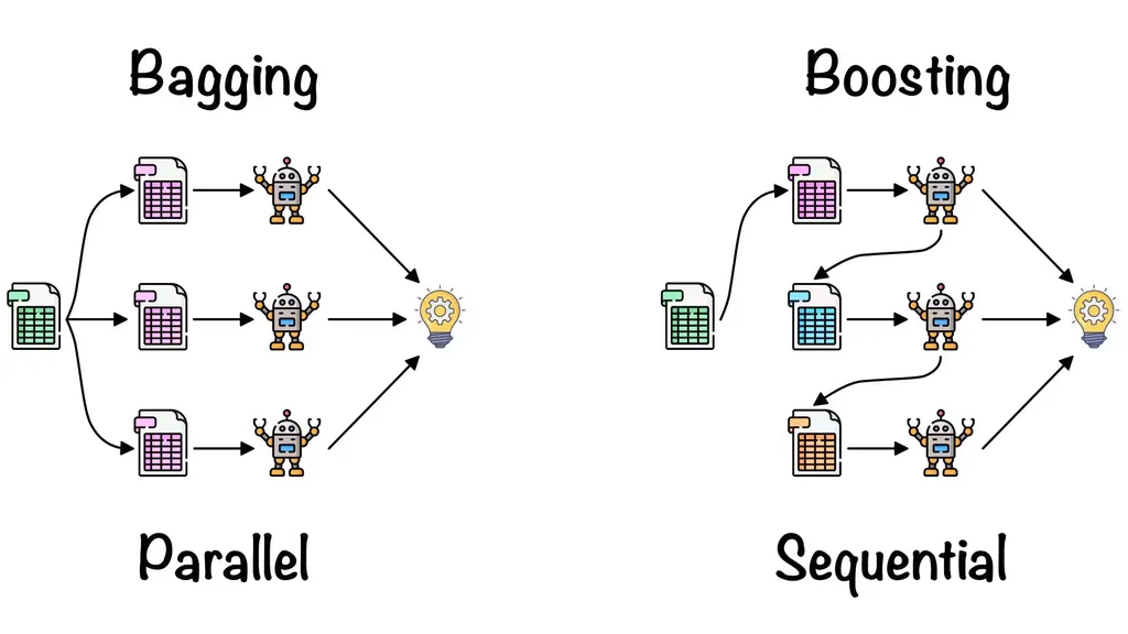
배깅(Bagging, Bootstrap Aggregating)

병렬적, 각각 독립적으로 학습, 결과 종합
학습 데이터를 무작위로 여러 부분 샘플(부트스트랩)로 나누어 각각 독립적으로 모델을 학습
예측 시에는 여러 모델의 결과를 평균(회귀) 혹은 다수결(분류)로 결정
(평균을 내서 최종 예측을 한다 = 회귀
가장 많은걸 선택해서 예측 = 분류)

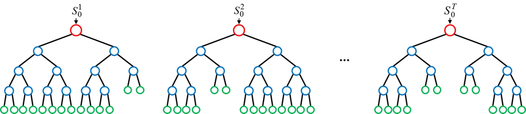
• 예시 : 랜덤포레스트(Random Forest), 분류/회귀 모두 가능
  
  like 스무고개

결정 트리 여러 개를 만들 때, 각 트리에 사용하는 피처와 데이터 샘플을 무작위로 선택 (피처 샘플링 + 데이터 샘플링)

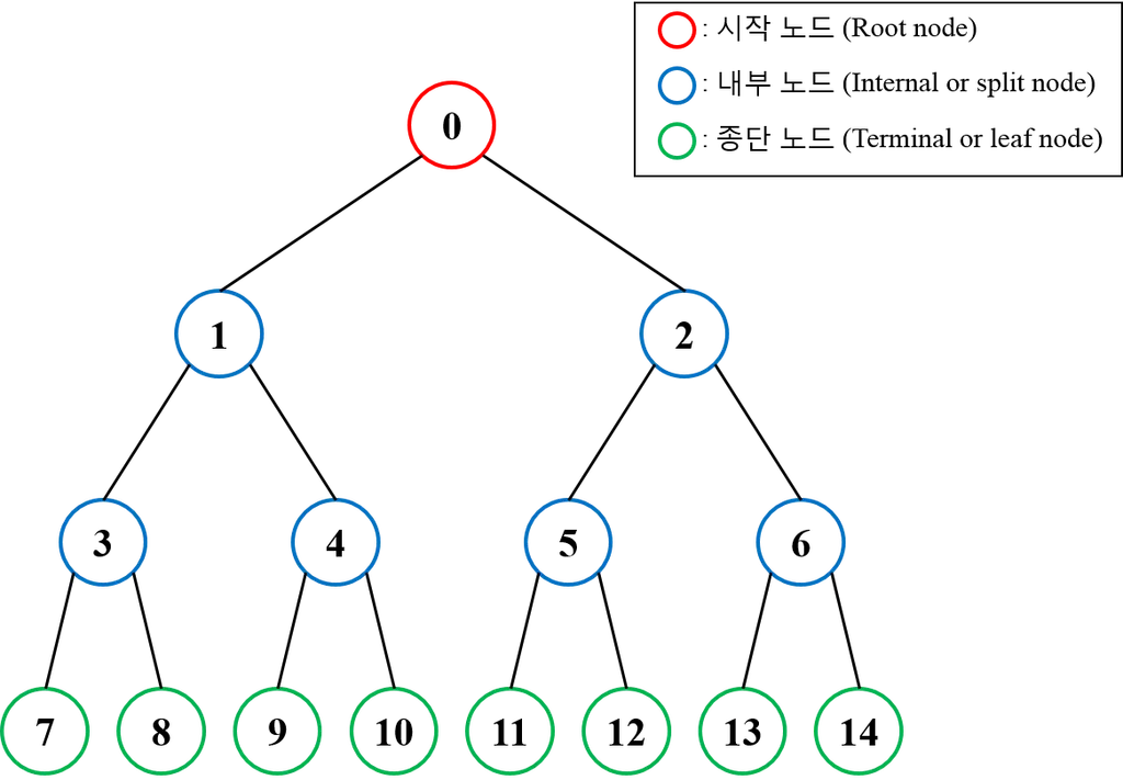
결정 트리(Decision Tree)는 데이터를 여러 조건(규칙)으로 분할하여 트리 형태로 예측을 수행하는 머신러닝 모델
트리기반 모델은 회귀와 분류 모두 할 수 있다.

장점

• 각 모델이 독립적으로 학습되므로 병렬 처리 가능 (학습 속도가 상대적으로 빠름)
• 모델 간 상호 간섭이 적어 안정적
• 과적합을 줄여주는 효과 (예측의 분산 감소, 모든 앙상블모델의 장점)

단점

• 많은 수의 모델을 학습해야 하므로 메모리 사용량이 많아질 수 있음
• 해석이 어려움(예측정확도와 해석은 반비례)

from sklearn.datasets import load_breast_cancer
from sklearn.model_selection import train_test_split
from sklearn.ensemble import RandomForestClassifier 
from sklearn.metrics import accuracy_score, confusion_matrix, classification_report

# 1. 데이터 로드
data = load_breast_cancer()
X = data.data
y = data.target

# 2. 학습/테스트 분할
X_train, X_test, y_train, y_test = train_test_split(
    X, y,
    test_size=0.2,
    random_state=42,
    stratify=y
)

# 3. 랜덤 포레스트 모델 생성
# n_estimators는 사용할 트리의 개수, max_depth는 각 트리의 최대 깊이를 의미하며
# 위 2개의 값을 높일 수록 시간과 연산량은 늘어나지만 더욱 복잡한 특징을 잡을 수 있음
rf_model = RandomForestClassifier(
    n_estimators=100,
    max_depth=None,
    random_state=42
)

# 4. 모델 학습
rf_model.fit(X_train, y_train)

# 5. 예측
y_pred = rf_model.predict(X_test)

# 6. 성능 평가
acc = accuracy_score(y_test, y_pred)
cm = confusion_matrix(y_test, y_pred)
report = classification_report(y_test, y_pred)

print(f"Accuracy: {acc:.4f}")
print("Confusion Matrix:\n", cm)
print("Classification Report:\n", report)

RandomForestClassifier , RandomForestregressor
종속변수만 연속적인 숫자로 하면 됨

load_breast_cancer()를 통해 이진분류용 유방암 진단 데이터셋을 불러온다. 데이터(X)와 라벨(y)을 분리.
train_test_split()으로 학습(train) 세트와 테스트(test) 세트를 8:2 비율로 분할.
random_state로 난수를 고정하고, 클래스 비율이 유지되도록 stratify=y를 지정.
n_estimators는 사용할 트리의 개수, max_depth는 각 트리의 최대 깊이
정확도(Accuracy), 혼동 행렬(Confusion Matrix), 분류 보고서(Classification Report)를 출력해 성능을 평가.
- accuracy_score()로 정확도.
- confusion_matrix()를 통해 실제 라벨 대비 예측 라벨의 분포
- classification_report()로 정밀도(precision), 재현율(recall), F1 점수 등 세부 지표를 확인

부스팅

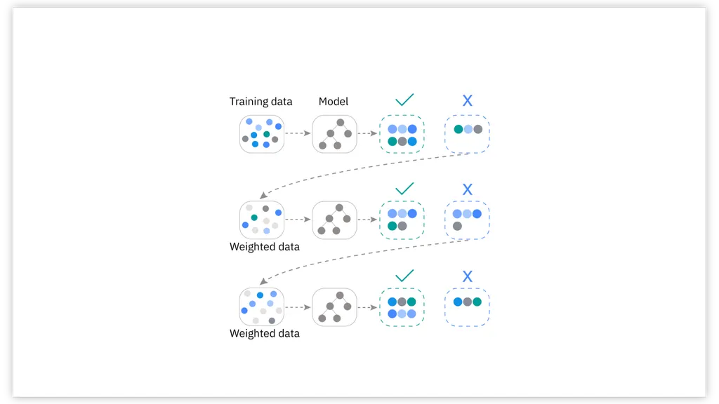
순차적으로 모델을 학습하면서 이전 모델이 만든 예측 오류를 보정하도록 설계
각각의 모델은 이전 모델이 틀린 부분에 가중치를 더 둬서 학습

대표 알고리즘

1. XGBoost (Extreme Gradient Boosting)
2. LightGBM
3. CatBoost

장점

• 높은 정확도 달성 가능
• 각 단계에서의 오류를 보정하기 때문에, 복잡한 데이터 패턴을 잘 포착

단점

순차적(Sequential)으로 학습하므로 병렬화가 쉽지 않음(속도측면)
하이퍼파라미터가 많고 튜닝이 까다롭다

• 작동 예시(XGBoost) 간단 시나리오

1. 기본 모델(약한 결정 트리) 훈련 → 예측 오류 확인
2. 예측 오류가 컸던 샘플에 높은 가중치 부여
3. 다음 모델(결정 트리) 훈련 → 다시 오류 보정
4. 이 과정을 여러 번 반복하여, 최종 예측 시에는 모두 합산

# 1. 데이터 준비 (Titanic 예시: 범주형 컬럼 존재)
from sklearn.datasets import fetch_openml
import pandas as pd
import numpy as np

# OpenML에서 Titanic 데이터셋 로드
titanic = fetch_openml('titanic', version=1, as_frame=True)
df = titanic.frame

df

# 주요 컬럼만 사용하고, 결측치가 있는 행 제거(XGB와 Light GBM을 위해)
# pclass(객실 등급, 범주형), sex(성별, 범주형), age(나이, 연속형), fare(티켓 요금, 연속형)
# embarked(탑승항구, 범주형), survived(생존 여부, 타깃)
df = df[['pclass', 'sex', 'age', 'fare', 'embarked', 'survived']]
df.dropna(inplace=True)

df

# 입력(X), 타깃(y) 분리
X = df.drop('survived', axis=1)
y = df['survived'].astype(int)  # survived 컬럼을 int형으로 변환

print(X.shape)
print(y.shape)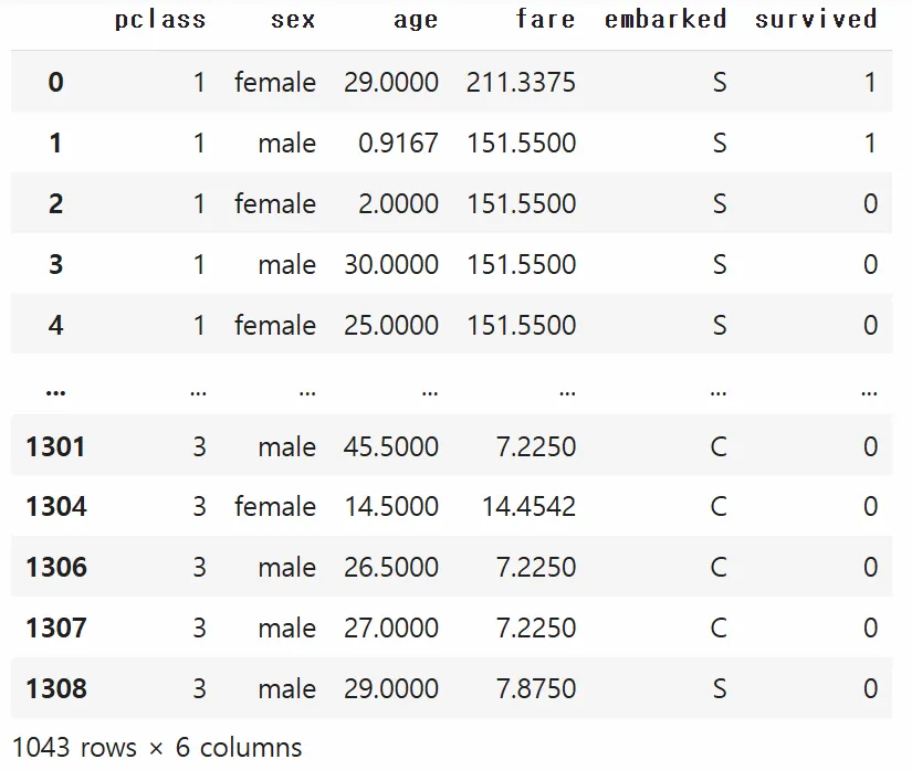

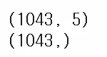
종속/독립 분리

# 2. 데이터 전처리
#    XGBoost/LightGBM은 숫자형 입력만 허용하므로, 범주형 칼럼을 인코딩
from sklearn.preprocessing import LabelEncoder

cat_cols = ['sex', 'embarked']  # 범주형으로 간주할 컬럼들
for col in cat_cols:
    le = LabelEncoder()
    X[col] = le.fit_transform(X[col])

X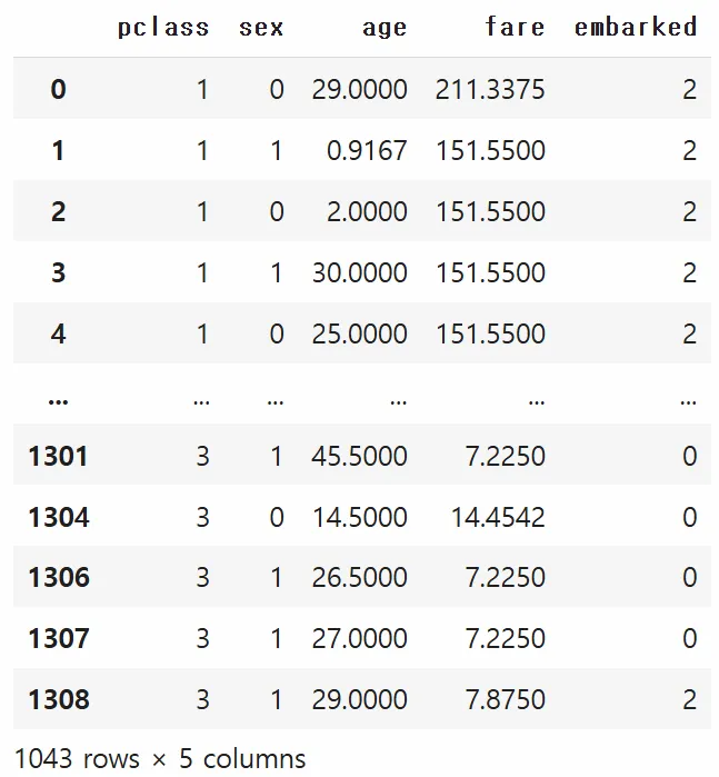

• 범주형 인코딩
  - XGBoost나 LightGBM은 입력을 숫자형으로만 처리하므로, LabelEncoder를 사용해 sex, embarked 등 범주형 컬럼들을 수치화.
  반복문을 이용해서 범주형 변수들을 자동으로 처리하게 함
  (사실 embarked는 원핫인코딩-순서가 없으면서 3가지 이상의 값을 갖는 경우-을 하는게 맞다 ~~ )

# 3. 학습/테스트 데이터 분할
from sklearn.model_selection import train_test_split

X_train, X_test, y_train, y_test = train_test_split(
    X, y,
    test_size=0.2,
    random_state=42,
    stratify=y
)

print(X_train.shape)
print(y_train.shape)
print(X_test.shape)
print(y_test.shape)

XGBoost

마찬가지 회귀, 분류 가능
XGBRegressor로 회귀 가능

# 4. XGBoost 실습
# (설치가 필요할 수 있습니다) ! pip install xgboost
from xgboost import XGBClassifier
from sklearn.metrics import accuracy_score, confusion_matrix, classification_report

xgb_model = XGBClassifier(random_state=42)
xgb_model.fit(X_train, y_train)
y_pred_xgb = xgb_model.predict(X_test)

print("=== XGBoost ===")
print("Accuracy:", accuracy_score(y_test, y_pred_xgb))
print("Confusion Matrix:\n", confusion_matrix(y_test, y_pred_xgb))
print("Classification Report:\n", classification_report(y_test, y_pred_xgb))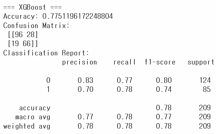

• XGBoost 실습
  • XGBClassifier를 생성 후 fit으로 학습
  • predict 결과와 실제값을 비교해 정확도, 혼동행렬, 분류 보고서를 출력

LightGBM

# 5. LightGBM 실습
# (설치가 필요할 수 있습니다) ! pip install lightgbm
from lightgbm import LGBMClassifier

lgb_model = LGBMClassifier(random_state=42)
lgb_model.fit(X_train, y_train)
y_pred_lgb = lgb_model.predict(X_test)

print("\n=== LightGBM ===")
print("Accuracy:", accuracy_score(y_test, y_pred_lgb))
print("Confusion Matrix:\n", confusion_matrix(y_test, y_pred_lgb))
print("Classification Report:\n", classification_report(y_test, y_pred_lgb))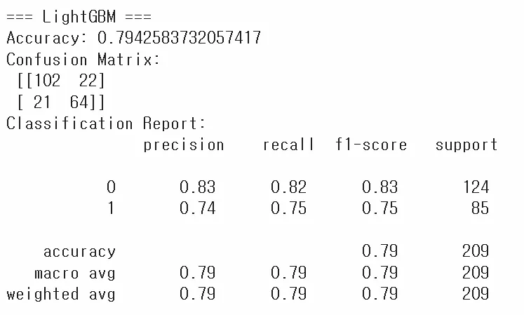

• LightGBM 실습
  • LGBMClassifier를 생성 후 동일한 절차로 학습/예측/평가

catboost

코랩사용자도 무조건 설치해야함

# 설치 필수!
! pip install catboost

# 6. CatBoost 실습 (범주형 특성 직접 지정 예시)
#    -> 별도의 인코딩 없이도 'cat_features' 인덱스를 지정 가능
# 이전 예시에선 이미 LabelEncoder로 숫자로 바꿨지만,
# CatBoost는 원본 범주형(문자열) 상태로도 학습 가능.

from catboost import CatBoostClassifier

# CatBoost용 데이터 준비: 원본 df에서 결측 제거(위에서 한 것 동일)
df_cat = titanic.frame[['pclass', 'sex', 'age', 'fare', 'embarked', 'survived']].dropna()
X_cat = df_cat.drop('survived', axis=1)
y_cat = df_cat['survived'].astype(int)

X_cat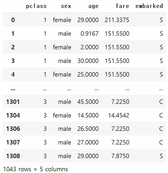

범주형 변수 그대로 있음

# cat_features 인덱스: 'sex', 'embarked' 컬럼(원본 df에서의 컬럼 인덱스)
# DataFrame 사용 시에는 컬럼 이름이 아니라 "열의 위치"를 지정해야 함
#   - pclass : 0, sex: 1, age: 2, fare: 3, embarked: 4
cat_features_idx = [1, 4]

X_cat_train, X_cat_test, y_cat_train, y_cat_test = train_test_split(
    X_cat, y_cat, test_size=0.2, random_state=42, stratify=y_cat
)

cat_model = CatBoostClassifier(
    cat_features=cat_features_idx,
    verbose=1,           # 학습과정 확인 가능
    random_state=42
)
cat_model.fit(X_cat_train, y_cat_train)
y_pred_cat = cat_model.predict(X_cat_test)

print("\n=== CatBoost ===")
print("Accuracy:", accuracy_score(y_cat_test, y_pred_cat))
print("Confusion Matrix:\n", confusion_matrix(y_cat_test, y_pred_cat))
print("Classification Report:\n", classification_report(y_cat_test, y_pred_cat))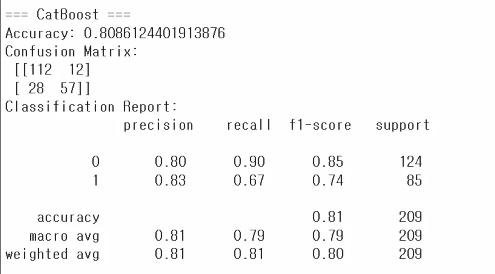

• CatBoost 실습
  - CatBoost는 범주형 데이터를 직접 지정(cat_features) 가능
  - 이를 위해 원본 DataFrame(문자열 범주형)을 다시 준비하고, cat_features 인덱스를 설정(카테고리 변수 설정)
  - CatBoostClassifier로 학습 후, 예측 결과를 평가
  verbose: 학습하는 과정을 볼 수 있게 함. 숫자만큼 학습할 때 마다 출력해줌
  

과적합 vs 과소적합

과적합

일반화가 안 된 상황
앙상블은 과적합 방지에 좋음(일반화가 잘 된 결론을 냄)
학습 데이터에는 지나치게 최적화되었지만, 새로운 데이터(테스트/실제 환경)에는 성능이 떨어지는 현상

원인

• 모델의 파라미터(자유도)가 너무 많아서 복잡도 과다(모델이 지나치게 복잡)
  특이한 데이터가 일부 존재할 수 있음

• 학습 데이터 수가 충분하지 않음

• 너무 많은 에폭(딥러닝 등)으로 학습
  에폭 = iteration, 반복횟수

• 노이즈가 많은 훈련 데이터에서 패턴을 ‘과하게’ 학습

해결방법

• 규제-정규화-(Regularization) 기법
  L1, L2 정규화 : 가중치(모델 파라미터)에 패널티를 줘서 과도한 학습 억제
  릿지/라쏘 등.
  penalty에 l1/l2 적용

• 드롭아웃(Dropout, 딥러닝에 주로 사용)
  학습 시 일부 뉴런을 확률적으로 비활성화 → 과적합 완화
  랜덤포레스트느낌.

• 데이터 증강(Data Augmentation)
  테크닉을 써서 데이터 수를 늘림
  - 이미지 데이터의 경우, 회전·이동·반전 등으로 새 데이터를 생성
  - 자연어 데이터에도 유사한 패턴으로 증강 가능
  - 신호 데이터의 경우 가우시안 노이즈를 추가하여 증강 가능

• 조기 종료(Early Stopping)
  학습 도중 검증 손실이 증가하기 시작하면 학습을 중단

• 앙상블(Ensemble)
  서로 다른 모델을 결합하여 과적합 위험을 줄임

과소적합

모델이 데이터의 패턴을 충분히 학습하지 못해, 학습 데이터조차도 충분히 맞추지 못하는 현상

해결방법

• 모델 복잡도 증가
• 더 오래 학습
• 모델 구조 변경 (더 깊은 신경망, 더 많은 트리 등)

하이퍼파라미터

파라미터는 모델이 정해주는 값(x앞에 붙는 값)
모델이 학습을 시작하기 전에 사람이 설정해야 하는 값 = 하이퍼 파라미터
ex) 결정 트리의 최대 깊이(max_depth), 학습 횟수 등

튜닝을 위한 준비

데이터셋 분할(Training/Validation/Test)

Training Set: 모델 학습에 직접 사용
Validation Set: 하이퍼파라미터 튜닝이나 모델 선택을 위해 사용
하이퍼파라미터 평가할 때 사용.
Test Set: 최종 성능 평가(훈련/검증 단계에 절대 포함되면 안 됨)

교차 검증(Cross-Validation)

데이터를 훈련 세트와 검증 세트(fold)로 여러 번 겹치지 않게 나누어 사용
장점: 데이터가 적은 상황에서도 안정적인 성능 평가 가능

• K-Fold Cross-Validation
  - 데이터를 K개의 폴드(Fold)로 나누어, 순차적으로 한 폴드를 검증 세트로 사용하고 나머지를 훈련에 사용
  데이터가 적을 때 주로 사용 but 개수가 많아지면 시간이 너무오래걸림
  - 평균 성능을 최종 모델의 성능으로 본다
  

튜닝 방법

1️⃣ Grid Search

• 미리 정의된 하이퍼파라미터 후보들의 ‘모든 조합’을 시도
• 장점: 완전 탐색이므로 최적값을 놓치지 않음
• 단점: 후보가 많아질수록 연산량이 급격히 증가

2️⃣ Randomized Search

• 임의로 샘플링된 하이퍼파라미터 조합을 일정 횟수만 시도
• 장점: 다양한 영역을 빠르게 탐색 가능, 속도 빠름
• 단점: 최적 조합을 정확히 찾지 못할 수도 있음

3️⃣ 베이지안 최적화(Bayesian Optimization)

어느정도 이유를 가지고 그럴싸한 조합을 가지고 시도

• 과거의 탐색 결과를 바탕으로 ‘가장 유망한 하이퍼파라미터 범위’를 중점적으로 탐색
• 장점: 탐색 시간이 더 짧고 효율적
• 단점: 구현 복잡도가 높음

Grid SearchCV 코드
cv = cross validation

from sklearn.datasets import load_iris
from sklearn.model_selection import train_test_split, GridSearchCV
from sklearn.ensemble import RandomForestClassifier
from sklearn.metrics import accuracy_score

# 1. 데이터 로드
iris = load_iris()
X = iris.data
y = iris.target

# 2. 학습/테스트 데이터 분할
X_train, X_test, y_train, y_test = train_test_split(
    X, y,
    test_size=0.2,
    random_state=42,
    stratify=y
)

# 3. 하이퍼 파라미터 후보군 설정
param_grid = {
    'n_estimators': [50, 100, 200],
    'max_depth': [None, 5, 10]
}

# 4. GridSearchCV 생성
rf = RandomForestClassifier(random_state=42)
grid_search = GridSearchCV(
    estimator=rf,
    param_grid=param_grid,
    cv=5,              # 교차검증(fold) 횟수
    scoring='accuracy',
    n_jobs=-1,          # 병렬 처리(가능한 모든 코어 사용)
)

# 5. 학습(그리드서치 수행)
grid_search.fit(X_train, y_train)

# 6. 최적 파라미터 및 성능 확인
print("Best Parameters:", grid_search.best_params_)
print("Best CV Score:", grid_search.best_score_)

# 7. 테스트 데이터 성능 확인
best_model = grid_search.best_estimator_
y_pred = best_model.predict(X_test)
test_acc = accuracy_score(y_test, y_pred)
print("Test Accuracy:", test_acc)

• stratify=y를 통해 클래스 비율이 유지되도록 함
• GridSearchCV를 생성
  • param_grid에 정의한 파라미터 후보군(param_grid)을 넣기.
  • cv=5로 5-Fold 교차검증을 수행.
  • scoring='accuracy'로 정확도를 기준으로 최적 파라미터를 찾기.
  • n_jobs=-1로 가능한 모든 CPU 코어를 사용해 계산을 병렬화.
• GridSearchCV로 학습.
  • fit(X_train, y_train)을 통해 주어진 파라미터 후보군 각각에 대해 모델을 학습하고 교차검증 성능을 비교.
  • 내부적으로 5-Fold 교차검증을 통해 파라미터 조합별 성능을 평가.
• 최적 파라미터와 교차검증 성능을 확인.
  • best_params_는 최고 성능을 낸 파라미터 조합.
  • best_score_는 교차검증에서의 최고 정확도.
• 테스트 세트로 최종 성능을 확인합니다.
  • best_estimator_는 최적 파라미터로 학습된 모델을 의미.
  • 테스트 세트 예측 결과로 정확도를 측정하여 모델의 최종 성능을 평가.

추가개념

최적화

• 하이퍼파라미터 튜닝(GridSearchCV, RandomizedSearchCV 등)
• 피처 엔지니어링(새로운 파생 변수 생성, 불필요한 변수 제거)
• 과적합 방지(교차검증, 규제 적용, 드롭아웃 등)

배포

• 학습 완료 모델을 운영 환경에 배포
• API 서버 구축, 클라우드(AWS, GCP) 또는 엣지 디바이스(임베디드 환경)
• 지속적 모니터링으로 모델 성능이 저하될 경우 재학습 주기 설정

MLOps(머신러닝 운영)

• Machine Learning + DevOps의 합성어
• 머신러닝 모델 개발부터 배포, 모니터링, 재학습, 롤백(Rollback) 등 전 과정을 자동화하고 효율적으로 운영하는 방법론
  프로젝트 완성 → 실제 운영 단계에서 지속적인 모니터링과 데이터/모델 업데이트가 필요

모델 해석 가능성(Explainable AI, XAI)

• 머신러닝, 특히 딥러닝 모델은 블랙박스처럼 동작
• 의료/금융 등 규제 산업에서는 “왜 이런 결과가 나왔는지”에 대한 설명 요구

주요기법

• LIME(Local Interpretable Model-agnostic Explanations)
• SHAP(Shapley Additive Explanations)
• Feature Importance 시각화(트리 기반 모델)

Feature Importance 코드 예시

import matplotlib.pyplot as plt
from sklearn.datasets import load_iris
from sklearn.model_selection import train_test_split
from sklearn.ensemble import RandomForestClassifier

# 1. 데이터 로드
iris = load_iris()
X = iris.data
y = iris.target
feature_names = iris.feature_names

# 2. 학습/테스트 데이터 분할
X_train, X_test, y_train, y_test = train_test_split(
    X, y,
    test_size=0.2,
    random_state=42,
    stratify=y
)

# 3. 랜덤 포레스트 모델 학습
rf = RandomForestClassifier(random_state=42)
rf.fit(X_train, y_train)

# 4. 피처 중요도 추출
importances = rf.feature_importances_

# 5. 시각화
plt.bar(range(len(importances)), importances)
plt.xticks(range(len(importances)), feature_names, rotation=45)
plt.xlabel("Feature")
plt.ylabel("Importance")
plt.title("Feature Importances in RandomForest")
plt.tight_layout()
plt.show()

# 가장 중요한 변수
most_important_idx = importances.argmax()
most_important_feature = feature_names[most_important_idx]
print("가장 중요한 변수:", most_important_feature)