
2-1 훈련 세트와 테스트 세트
학습 목표
- 지도 학습과 비지도 학습의 차이를 배운다.
- 모델을 훈련시키는 훈련 세트와 모델을 평가하기 위한 테스트 세트로 데이터를 나눠서 학습해보자.
1) 지도 학습과 비지도 학습
📕 개념 정리
알고리즘은 크게 지도 학습과 비지도 학습으로 나뉜다.
- 지도 학습 : 입력(input)과 정답(target) 데이터를 사용하여 학습
- 비지도 학습 : 정답이 없이 입력 데이터만 사용하여 학습
* 강화학습 (reinforcement learning) : target이 아닌 알고리즘이 행동한 결과로 얻은 보상을 활용하여 학습
2) train set과 test set
📕 샘플 생성(생선 전체의 길이, 무게, 타겟 데이터 생성)
fish_length = [25.4, 26.3, 26.5, 29.0, 29.0, 29.7, 29.7, 30.0, 30.0, 30.7, 31.0, 31.0,
                31.5, 32.0, 32.0, 32.0, 33.0, 33.0, 33.5, 33.5, 34.0, 34.0, 34.5, 35.0,
                35.0, 35.0, 35.0, 36.0, 36.0, 37.0, 38.5, 38.5, 39.5, 41.0, 41.0, 9.8,
                10.5, 10.6, 11.0, 11.2, 11.3, 11.8, 11.8, 12.0, 12.2, 12.4, 13.0, 14.3, 15.0]
fish_weight = [242.0, 290.0, 340.0, 363.0, 430.0, 450.0, 500.0, 390.0, 450.0, 500.0, 475.0, 500.0,
                500.0, 340.0, 600.0, 600.0, 700.0, 700.0, 610.0, 650.0, 575.0, 685.0, 620.0, 680.0,
                700.0, 725.0, 720.0, 714.0, 850.0, 1000.0, 920.0, 955.0, 925.0, 975.0, 950.0, 6.7,
                7.5, 7.0, 9.7, 9.8, 8.7, 10.0, 9.9, 9.8, 12.2, 13.4, 12.2, 19.7, 19.9]

fish_data = [[l,w] for l,w in zip(fish_length, fish_weight)]

fish_target = [1]*35 + [0]*14
📕 train, test set 생성 및 훈련
from sklearn.neighbors import KNeighborsClassifier
kn = KNeighborsClassifier()

# train set 생성(처음 35개 활용)
train_input = fish_data[:35]
train_target = fish_target[:35]

# test set 생성(마지막 14개 활용)
test_input = fish_data[35:]
test_target = fish_target[35:]

# test 훈련
kn.fit(train_input,train_target)
3) 샘플링 편향
📕 결과 확인
# 모델 평가
kn.score(test_input,test_target)
▶ 0.0
❗ discussion
모델 평가 점수가 0점이 나왔다.
훈련시켜준 데이터가 전부 도미로 편향되어있기 때문이다.
이를 샘플링 편향이라고 하며, 샘플링 편향을 방지하기 위해서는
여러 타겟을 지닌 데이터를 고루 섞어서 훈련시켜야 한다.
4) Numpy 활용한 랜덤 샘플링
📕 Numpy란?
파이썬의 대표적인 array 라이브러리로, 고차원의 배열을 쉽고 간편하게 만들 수 있다.
📕 Numpy 활용 array 생성
- numpy import 및 배열 생성
import numpy as np
input_arr = np.array(fish_data)
target_arr = np.array(fish_target)

print(input_arr)
▶
[[  25.4  242. ]
 [  26.3  290. ]
 [  26.5  340. ]
 [  29.   363. ]
 ...
- array 가 아닌 동일한 list 출력
print(fish_data)
▶
[[25.4, 242.0], [26.3, 290.0], [26.5, 340.0], [29.0, 363.0],...
❗ discussion
list와 array의 내용은 동일하나,
일반적인 list와 다르게 array는 행과 열을 알기 쉽게 출력해주며,
배열의 크기를 알려주는 shape 속성을 제공한다.
print(input_arr.shape)
▶
(49, 2)
📕 랜덤하게 샘플을 선택하여 train, test set 생성
동일한 생선의 데이터가 들어가야하므로 input_arr과 target_arr의 위치는 함께 선택되어야함
따라서 0~48까지의 index를 랜덤하게 섞고 해당 index에 따른 input, target을 뽑아내자
np.random.seed(42)          # random 함수에 시드 지정
index = np.arange(49)       # 0부터 n-1까지 1씩 증가하는 배열
np.random.shuffle(index)    # 무작위로 섞어줌
▶
array([13, 45, 47, 44, 17, 27, 26, 25, 31, 19, 12,  4, 34,  8,  3,  6, 40,
       41, 46, 15,  9, 16, 24, 33, 30,  0, 43, 32,  5, 29, 11, 36,  1, 21,
        2, 37, 35, 23, 39, 10, 22, 18, 48, 20,  7, 42, 14, 28, 38])

# train set 생성
train_input = input_arr[index[:35]]
train_target = target_arr[index[:35]]

# test set 생성
test_input = input_arr[index[35:]]
test_target = target_arr[index[35:]]
📕 scatter plot으로 data set 살펴보기
import matplotlib.pyplot as plt
plt.figure(figsize = (10,10))
plt.scatter(train_input[:,[0]],train_input[:,[1]], label='train')
plt.scatter(test_input[:,[0]],test_input[:,[1]], label='target')
plt.xlabel('length')
plt.ylabel('weight')
plt.legend()
plt.show();- 결과이미지
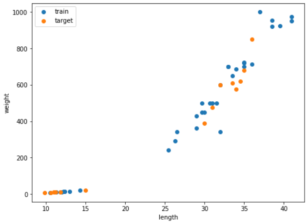
❗ discussion
train set과 test set 모두에 도미(우측상단)와 빙어(좌측하단) 데이터가 잘 섞인 것을 확인할 수 있다.
5) 모델 검증
📕 앞서 만든 data set으로 k-최근접 이웃 모델 훈련
# 클래스 객체 생성
kn = KNeighborsClassifier()

# 모델 훈련
kn.fit(train_input,train_target)

# 모델 평가
kn.score(test_input, test_target)
▶
1.0

# 모델 활용 예측
kn.predict(test_input)
▶
array([0, 0, 1, 0, 1, 1, 1, 0, 1, 1, 0, 1, 1, 0])

# test_target에 비교 확인
print(test_target)
▶
array([0, 0, 1, 0, 1, 1, 1, 0, 1, 1, 0, 1, 1, 0])- 결과
모델 평가 score도 100%이며,
실제 test set의 예측 결과와 test target이 일치하는 것을 알 수 있다.
❗ discussion
predict() 메서드가 반환하는 값은 list가 아니라 numpy array이다.
사이킷런 모델의 표준 데이터는 numpy data이다.
📕 키워드 정리
지도학습이란
- 입력과 target을 전달하여 훈련한 다음 새로운 데이터의 target을 예측하는 학습방법
비지도학습
- target 데이터 없이 진행하는 학습으로, 무엇을 예측하는 것이 아닌 입력 데이터에서 어떤 특징을 찾는데 활용된다.
2-2 데이터 전처리
학습 목표
- 올바른 결과 도출을 위해서 데이터를 사용하기 전에 데이터 전처리 과정을 거친다.
- 전처리 과정을 거친 데이터로 훈련했을 때의 차이를 알고, 표준점수로 특성의 스케일을 변환하는 방법을 배운다.
1) Numpy로 데이터 준비하기
📕 input 데이터 numpy 배열 만들기
fish_length = [25.4, 26.3, 26.5, 29.0, 29.0, 29.7, 29.7, 30.0, 30.0, 30.7, 31.0, 31.0,
                31.5, 32.0, 32.0, 32.0, 33.0, 33.0, 33.5, 33.5, 34.0, 34.0, 34.5, 35.0,
                35.0, 35.0, 35.0, 36.0, 36.0, 37.0, 38.5, 38.5, 39.5, 41.0, 41.0, 9.8,
                10.5, 10.6, 11.0, 11.2, 11.3, 11.8, 11.8, 12.0, 12.2, 12.4, 13.0, 14.3, 15.0]
fish_weight = [242.0, 290.0, 340.0, 363.0, 430.0, 450.0, 500.0, 390.0, 450.0, 500.0, 475.0, 500.0,
                500.0, 340.0, 600.0, 600.0, 700.0, 700.0, 610.0, 650.0, 575.0, 685.0, 620.0, 680.0,
                700.0, 725.0, 720.0, 714.0, 850.0, 1000.0, 920.0, 955.0, 925.0, 975.0, 950.0, 6.7,
                7.5, 7.0, 9.7, 9.8, 8.7, 10.0, 9.9, 9.8, 12.2, 13.4, 12.2, 19.7, 19.9]

fish_data = np.column_stack((fish_length, fish_weight))
▶
array([[  25.4,  242. ],
       [  26.3,  290. ],
       [  26.5,  340. ],
       [  29. ,  363. ],
       [  29. ,  430. ],
       ......
📕 target 데이터 numpy 배열 만들기
fish_target = np.concatenate((np.ones(35), np.zeros(14)))
print(fish_target)
▶
[1. 1. 1. 1. 1. 1. 1. 1. 1. 1. 1. 1. 1. 1. 1. 1. 1. 1. 1. 1. 1. 1. 1. 1.
 1. 1. 1. 1. 1. 1. 1. 1. 1. 1. 1. 0. 0. 0. 0. 0. 0. 0. 0. 0. 0. 0. 0. 0.
 0.]
❗ discussion
numpy의 column_stack()이나 concatenate() 메서드 사용 시 연결한 리스트나 배열을 튜플로 전달해야한다.
📕 scikitlearn으로 train set, test set 나누기
from sklearn.model_selection import train_test_split
train_input, test_input, train_target, test_target = train_test_split(fish_data, fish_target, random_state=42)

datas = [train_input, test_input, train_target, test_target]
for data in datas :
    print(data.shape)
▶
(36, 2)
(13, 2)
(36,)
(13,)

print(test_target)
▶
[1. 0. 0. 0. 1. 1. 1. 1. 1. 1. 1. 1. 1.]- 결과
train set과 test set이 input, target의 경우에 각각의 데이터 수가 똑같음을 알 수 있다.
❗ discussion
numpy의 tratin_test_split() 메서드는 기본적으로 전체의 25%를 test set으로 떼어낸다.
test target data set의 경우 13개 중 1이 10개, 0이 3개로 약간의 샘플링 편향이 나타나는 것으로 보인다.
원래의 비율은 35:14로 2.5:1 이나 해당 test set에서는 3.3:1이다.
📕 stratify 매개변수 활용 샘플링 편향 최소화
train_input, test_input, train_target, test_target = train_test_split(fish_data, fish_target, stratify=fish_target, random_state=42)

from collections import Counter
Counter(test_target)
▶
Counter({0.0: 4, 1.0: 9})- 결과
test target data set의 경우 13개 중 1이 9개, 0이 4개로 2.25:1의 비율을 보인다.
❗ discussion
stratify 활용 시 실제 target 비율(2.5:1)에 가까운 2.25:1의 비율로 샘플을 split 할 수 있었다.
데이터가 작아 전체 train data의 비율과 동일하게 맞출 수는 없지만,
train data가 작거나 특정 class의 샘플 개수가 적을 때 유용한 방법이다.
2) 이상치 확인
📕 앞서 준비한 data set으로 모델 생성
# 모델 생성
from sklearn.neighbors import KNeighborsClassifier
kn = KNeighborsClassifier()

# train set 훈련
kn.fit(train_input, train_target)

# test set 평가
kn.score(test_input, test_target)
▶
1.0- 결과
train data set 으로 훈련한 모델을 통해 test data set 검증 시 모든 데이터가 옳게 검증되었다.
📕 이상치 data 기존 모델 예측
kn.predict([[25,150]])
▶
array([0.])- 결과
도미(1) 데이터를 넣고 예측하였더니 정확도가 100%인 모델이 0이라는 틀린 결과를 도출하였다.
📕 이상치 data scatter plot 확인
import matplotlib.pyplot as plt
plt.figure(figsize = (8,6))
plt.scatter(train_input[:,0], train_input[:,1], label = 'train set')
plt.scatter(25, 150, marker='^', label = 'outlier')
plt.xlabel('length')
plt.ylabel('weight')
plt.legend()
plt.show();- 결과이미지
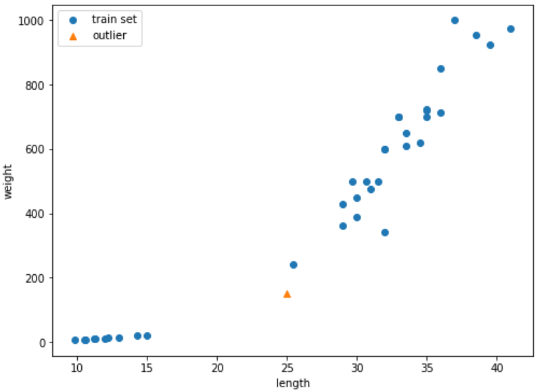
❗ discussion
이상치 마커의 위치는 왼쪽 하단 빙어 데이터보다는 우측 상단 도미 데이터에 더 가깝다.
k-최근접 이웃 모델은 주변의 샘플 중에서 다수인 클래스를 예측으로 사용한다.
📕 kneibors() 메서드 활용 이상치 주변 데이터 확인
1) 인근 5개 데이터 추출
distances, indexes = kn.kneighbors([[25,150]])
print(distances, indexes)
▶
[[ 92.00086956 130.48375378 130.73859415 138.32150953 138.39320793]] [[21 33 19 30  1]]
2) scatter plot 그리기
plt.figure(figsize = (8,6))
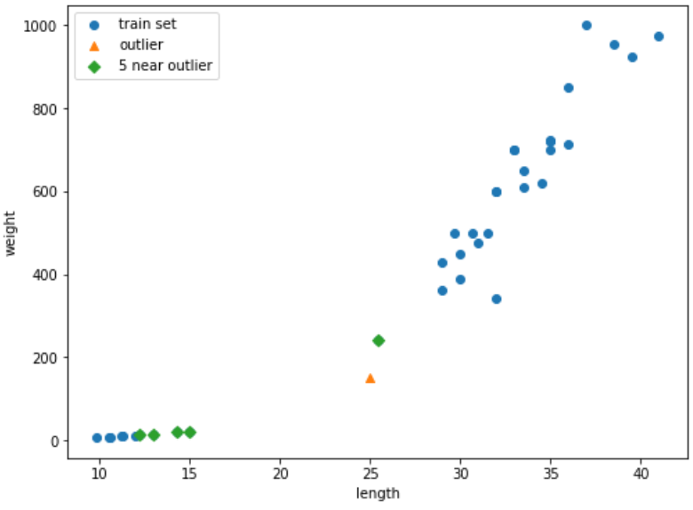
plt.scatter(train_input[:,0], train_input[:,1], label = 'train set')
plt.scatter(25, 150, marker='^', label = 'outlier')
plt.scatter(train_input[indexes,0], train_input[indexes,1], label = 'around outlier')
plt.xlabel('length')
plt.ylabel('weight')
plt.legend()
plt.show();- 결과 이미지
3) 인근 데이터 확인
# length, weight 확인
print(train_input[indexes])
▶
[[[ 25.4 242. ]
  [ 15.   19.9]
  [ 14.3  19.7]
  [ 13.   12.2]
  [ 12.2  12.2]]]

# target 확인
print(train_target[indexes])
▶
[[1. 0. 0. 0. 0.]]

# 거리 확인
print(distances)
[[ 92.00086956 130.48375378 130.73859415 138.32150953 138.39320793]]
❗ discussion
scatter plot과 target 값에서 확인 가능하듯이 이상치와 가까운 생선 4개는 빙어(0)이다.
그런데 scatter plot으로는 직관적으로 도미(1)과 더 가까워 보인다.
또한 distance 상으로 확인했을 때 거리 비율에 비해 scatter plot 상의 거리 비율은 훨씬 이상하다.
이는 그래프 비율이 4:3 인 것과 가로, 세로축의 간격 차이로 인해 발생한 것으로 보인다.
📕 그래프 비율 조절을 통한 직관성 높이기
plt.figure(figsize = (8,8))  # 그래프 비율 1:1
plt.scatter(train_input[:,0], train_input[:,1], label = 'train set')
plt.scatter(25, 150, marker='^', label = 'outlier')
plt.scatter(train_input[indexes,0], train_input[indexes,1], marker='D', label = '5 near outlier')
plt.xlim((0,1000))           # x축 범위 지정
plt.xlabel('length')
plt.ylabel('weight')
plt.legend()
plt.show();- 결과이미지
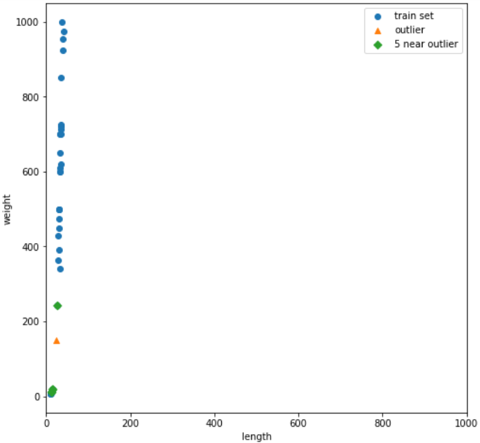
❗ discussion
두개 축의 범위를 동일하게 맞추었더니 데이터가 일직선으로 늘어선다.
무게에 비해 길이는 가까운 데이터를 찾는데 크게 영향을 미치지 못한다.
두 특성의 scale 이 다르기 때문이다.
3) 스케일링
📕 표준점수를 활용한 스케일링
표준 점수(z 점수)란?
각 특성값이 평균에서 표준편차의 몇 배만큼 떨어져 있는지를 나타낸다.
이를 통해 실제 특성값의 크기와 상관없이 동일한 조건으로 비교할 수 있다.
개별 데이터의 특성값에서 평균을 빼준 후 표준편차로 나누어 주면 된다.
# 각 열마다 특성 데이터가 있으므로 행을 따라(axis = 0) 각 열의 통계 값을 계산한다.
mean = np.mean(train_input, axis= 0)
std = np.std(train_input, axis=0)

print(mean, std)
▶
[ 27.29722222 454.09722222] [  9.98244253 323.29893931]

# numpy 브로드캐스팅 기능 활용
train_scaled = (train_input-mean)/std
📕 scatter plot by scaled data
new = ([25,150]-mean)/std

plt.figure(figsize = (8,8))
plt.scatter(train_scaled[:,0], train_scaled[:,1], label='train set')
plt.scatter(new[0], new[1], marker='^', label='outlier')
plt.xlabel('length')
plt.ylabel('weight')
plt.legend()
plt.show()- 결과이미지
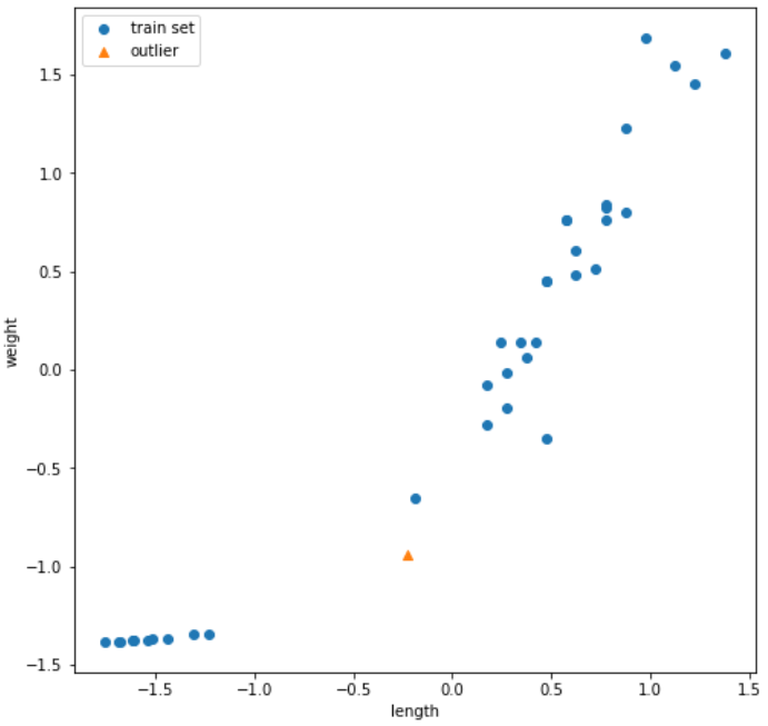
❗ discussion
스케일링 이전의 scatter plot과 유사하나, 두개의 축의 범위가 -1.5~1.5로 변경 되었다.
4) 전처리 데이터로 모델 생성
📕 전처리 데이터 활용 훈련 및 평가
# 모델 생성
kn.fit(train_scaled, train_target)

# test set 스케일링
test_scaled = (test_input-mean)/std

# test set 평가
kn.score(test_scaled, test_target)
▶
1.0

# 이상치 예측
kn.predict([new])
▶
array([1.])- 결과
모든 테스트 샘플을 완벽하게 분류하였고,
이상치 또한 정확히 분류하여 더이상 이상치가 아니게 되었다.
📕 전처리 데이터 활용 이웃 데이터 확인
distances, indexes = kn.kneighbors([new])

plt.figure(figsize = (8,8))
plt.scatter(train_scaled[:,0], train_scaled[:,1], label='train set')
plt.scatter(new[0], new[1], marker='^', label='outlier')
plt.scatter(train_scaled[indexes,0], train_scaled[indexes,1], marker='D', label='5 near outlier')
plt.xlabel('length')
plt.ylabel('weight')
plt.legend()
plt.show()- 결과이미지
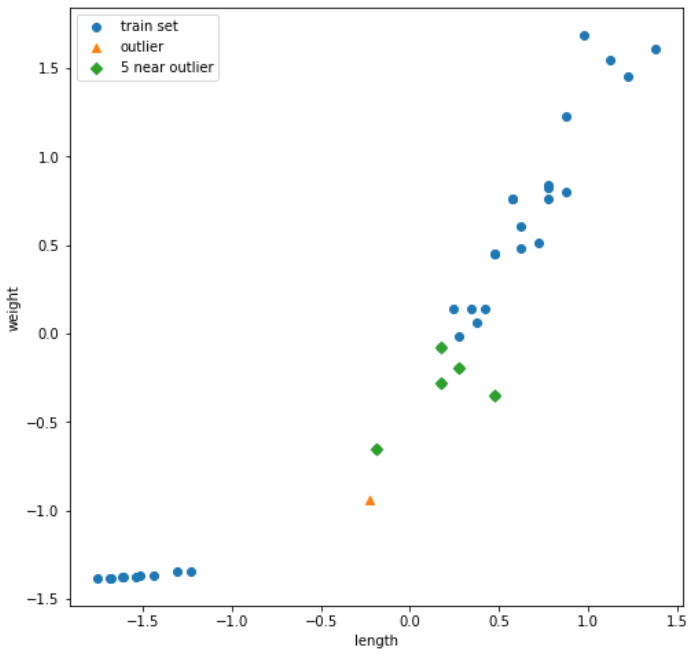
❗ discussion
이상치 인근의 5개 데이터 모두 도미로 정상적으로 나오는 것을 확인하였다!
📕 키워드 정리
데이터 전처리
- 머신러닝 모델에 훈련 데이터를 주입하기 전에 가공하는 단계
표준점수
- train set의 스케일을 바꾸는 대표적인 방법 중 하나이다.
- 표준점수 = (특성값 - 평균 특성값)/표준편차
- train과 test set 모두 스케일링 해주어야 하며,
반드시 train set의 평균과 표준 편차로 test set 스케일링을 진행해야함
브로드캐스팅
- 크기가 다른 numpy array에서 자동으로 사칙 연산을 모든 행이나 열로 확장하여 수행하는 기능
