Importing Matplotlib

# In[1]
import matplotlib as mpl
import matplotlib.pyplot as plt

Setting Styles

• We will use plt.style directive to choose appropriate aesthetic styles for our figures.
• We will set the classic style, which ensures that the plots we create use the classic Matplotlib style.

# In[2]
plt.style.use('classic')

How to Display Your Plots

• A visualization you can't see won't be of much use, but just how you view your Matplotlib plots depends on the context.
• The best use of Matplotlib differs depending on how you are using it; the three applicable contexts are using Matplotlib in a script, in an IPython terminal, or in a Jupyter notebook.

Plotting from a Script

• If you are using Matplotlib from within a script, plt.show is very important function.
• It starts an event loop, looks for all currently active Figure objects, and opens one or more interactive windows that display your figure or figures.

# In[3]
# file: myplot.py
import matplotlib.pyplot as plt
import numpy as np

x=np.linspace(0,10,100)

plt.plot(x,np.sin(x))
plt.plot(x,np.cos(x))

plt.show()

• You can run this script from the command-line prompt, which will result in a window opening with your figure displayed: $ python myplot.py
• The plt.show command should be used only once per Python session, and is most often seen at the very end of the script.

Plotting from an IPython Shell

• IPython is built to work well with Matplotlib if you specify Matplotlib mode.
• To enable this mode, you can use the %matplotlib command after starting ipython.
• At this point, any plt plot command will cause a figure window to open, and further commands can be run to update the plot.
• Some changes will not draw automatically. To force an update, use plt.draw.
• Using plt.show in IPython's Matplotlib mode is not required.

Plotting from a Jupyter Notebook

• Plotting interactively within a Jupyter notebook can be done with the %matplotlib command and works in a similar way to the IPython shell.
• You also have the option of embedding graphics directly in the notebook, with two possible options.
  • %matplotlib inline will lead to static images of your plot embedded in the notebook.
  • %matplotlib notebook will lead to interactive plots embedded within the notebook

# In[4]
%matplotlib inline
x=np.linspace(0,10,100)

fig=plt.figure()
plt.plot(x,np.sin(x),'-')
plt.plot(x,np.cos(x),'--');

Saving Figures to File

• One feature of Matplotlib is the ability to save figures in a wide variety of formats.
• Saving the figure can be done using the savefig command.

# In[5]
fig.savefig('my_figure.png')

• We now have a file called my_figure.png in the current working directory.
• To confirm that it contains what we think it contains, we can use the IPython Image object to display the contents of this file.

# In[6]
from IPython.display import Image
Image('my_figure.png')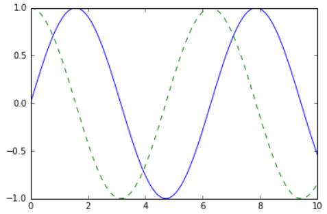

• In savefig, the file format is inferred from the extension of the given filename.
• Depending on what backends you have installed, many different file formats are available.
• The list of supported file types can be found for your system like this.

# In[7]
fig.canvas.get_supported_filetypes()

# Out[7]
{'eps': 'Encapsulated Postscript',
 'jpg': 'Joint Photographic Experts Group',
 'jpeg': 'Joint Photographic Experts Group',
 'pdf': 'Portable Document Format',
 'pgf': 'PGF code for LaTeX',
 'png': 'Portable Network Graphics',
 'ps': 'Postscript',
 'raw': 'Raw RGBA bitmap',
 'rgba': 'Raw RGBA bitmap',
 'svg': 'Scalable Vector Graphics',
 'svgz': 'Scalable Vector Graphics',
 'tif': 'Tagged Image File Format',
 'tiff': 'Tagged Image File Format'}

Two Interfaces for the Price of One

MATLAB-style Interface

• The MATLAB-style tools are contained in the pyplot(plt) interface.

# In[8]
plt.figure()

# create the first of two panels and set current axis
plt.subplot(2,1,1)
plt.plot(x,np.sin(x))

# create the second panel and set current axis
plt.subplot(2,1,2)
plt.plot(x,np.cos(x))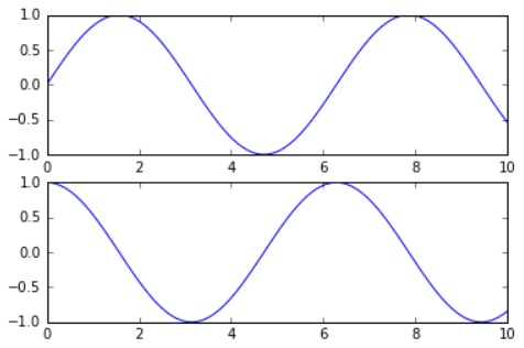

• It is important to recognize that this interface is stateful: it keeps track of the 'current' figure and axes, which are where all plt commands are applied.
• You can get a reference to these using the plt.gcf (get current figure) and plt.gca (get current axes) routines.

Object-oriented interface

• The object-oriented interface is available for these more complicated situations, and for when you want more control over your figure.
• Rather than depending on some notion of an active figure or axes, in the object-oriented interface the plotting functions are methods of explicit Figure and Axes objects.

# In[9]
# First create a grid of plots
# ax will be an array of two Axes objects
fig, ax=plt.subplots(2)

# Call plot() method on the appropriate object
ax[0].plot(x,np.sin(x))
ax[1].plot(x,np.cos(x));

• For simpler plots, the choice of which style to use is largely a matter of preference, but the object-oriented approach can become a necessity as plots become more complicated.