10주차 6차 미니프로젝트 (1차)

정지원·2024년 5월 1일

에이블 스쿨 복습

목록 보기

41/51

주제: '유통 판매량 예측 및 재고 최적화'
1. 데이터 탐색 및 가설 도출
2. 데이터 전처리 및 base_line_modeling

이 단계를 3일에 걸쳐서 진행합니다.

유통 판매량 예측 및 재고 최적화를수행하는 핵심 대상 상품

대상 상품(핵심 상품)

Product_ID	Product_Code	SubCategory	Category	LeadTime	Price
3	DB001	Beverage	Drink	2	8
12	GA001	Milk	Food	3	6
42	FM001	Agricultural products	Grocery	3	5

44번 매장의 상품번호 3, 12, 42 세가지 항목을 정하여 진행하였습니다.

변수 소개

oil_price 상위 5개 항목

	Date	WTI_Price
0	2014-01-01	NaN
1	2014-01-02	95.14
2	2014-01-03	93.66
3	2014-01-06	93.12
4	2014-01-07	93.31

orders 상위 5개 항목

	Date	Store_ID	CustomerCount
0	2014-01-01	25	840
1	2014-01-01	36	487
2	2014-01-02	1	1875
3	2014-01-02	2	2122
4	2014-01-02	3	3350

sales 상위 5개 항목

	Date	Store_ID	Product_ID
0	2014-01-01	1	3
1	2014-01-01	1	5
2	2014-01-01	1	7
3	2014-01-01	1	8
4	2014-01-01	1	10

products 상위 5개 항목

	Product_ID	Product_Code	SubCategory	Category	LeadTime	Price
0	20	HG001	Gardening Tools	Household Goods	2	50
1	27	HH001	Home Appliances	Household Goods	2	150
2	16	HK001	Kitchen	Household Goods	2	23
3	15	HK002	Kitchen	Household Goods	2	41
4	32	GS001	Seafood	Grocery	3	34

stores 상위 5개 항목

	Store_ID	City	State	Store_Type
0	1	Saint Paul	\tMinnesota	4
1	2	Saint Paul	\tMinnesota	4
2	3	Saint Paul	\tMinnesota	4
3	4	Saint Paul	\tMinnesota	4
4	5	Oklahoma City	Oklahoma	4

1. 데이터 탐색 및 가설 도출

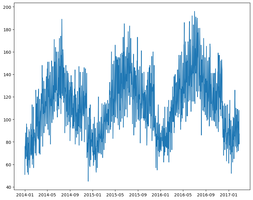
매장(44번)의 대상 상품의 판매량 추이

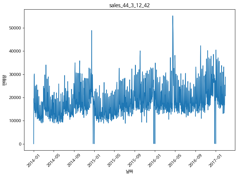
PRODUCT_ID - 3

시계열 패턴 1

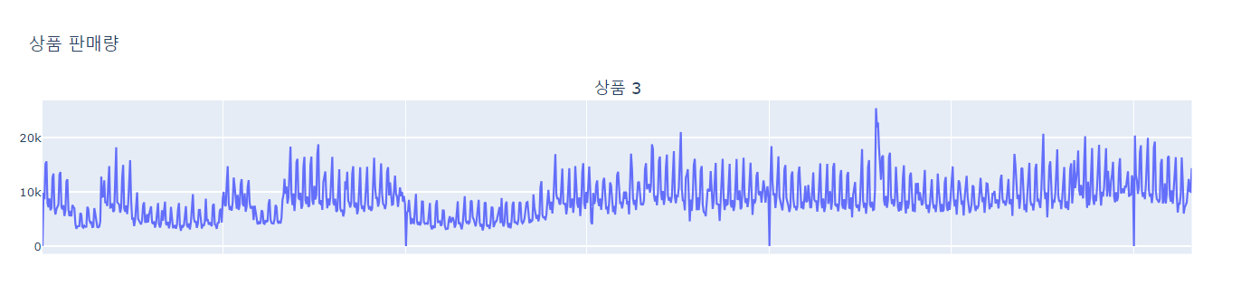
3번 상품의 동일 카테고리의 상품별 판매량 추이
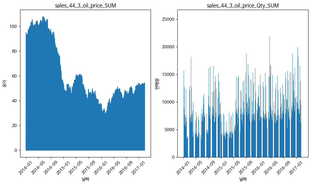
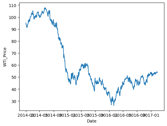
휘발유 가격과 상품 판매량 추이 비교

시계열 패턴 2

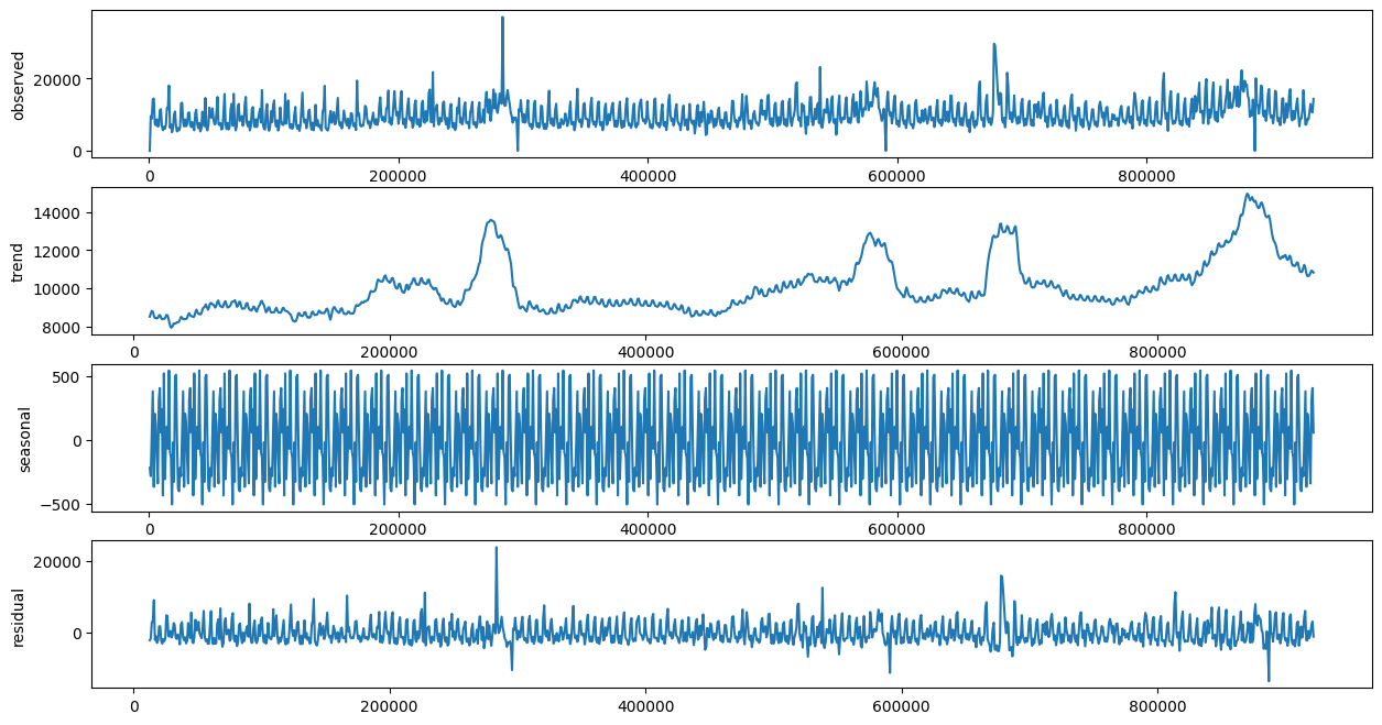
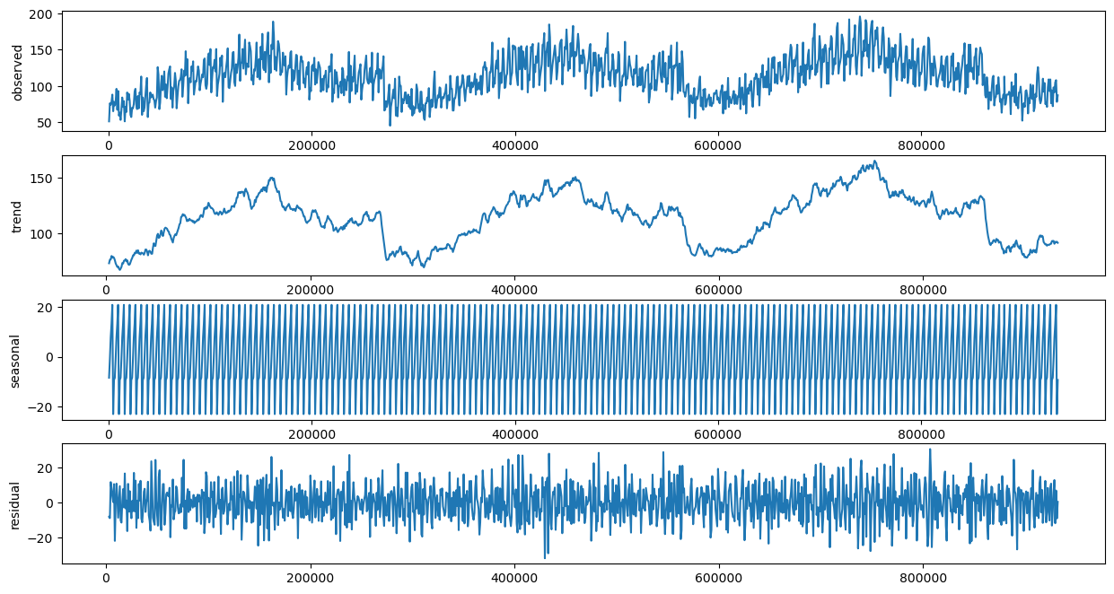
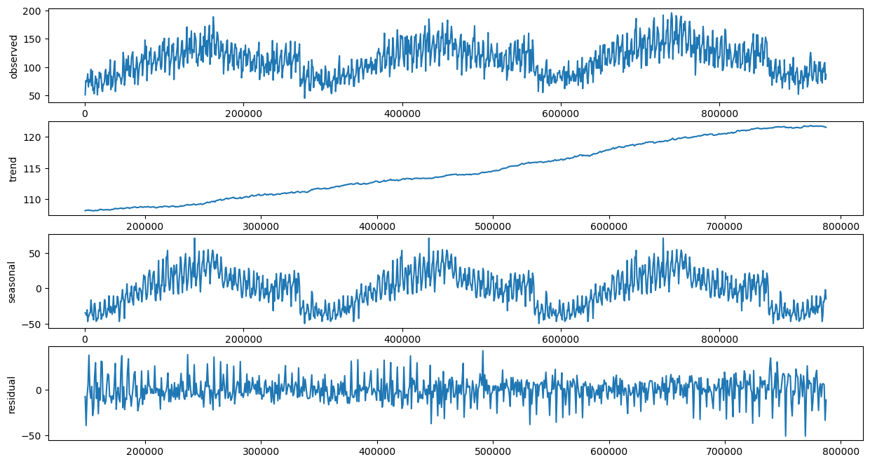
시계열 데이터 분해 (30일 주기)
시계열 데이터 분해 (365일 주기)

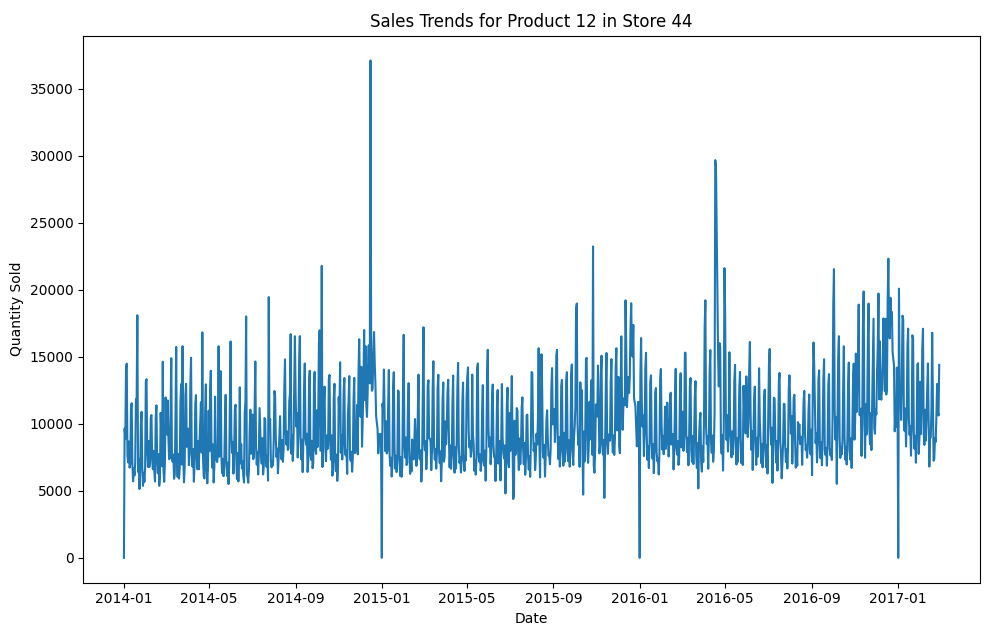
PRODUCT_ID - 12

시계열 패턴 1

12번 상품의 동일 카테고리의 상품별 판매량 추이

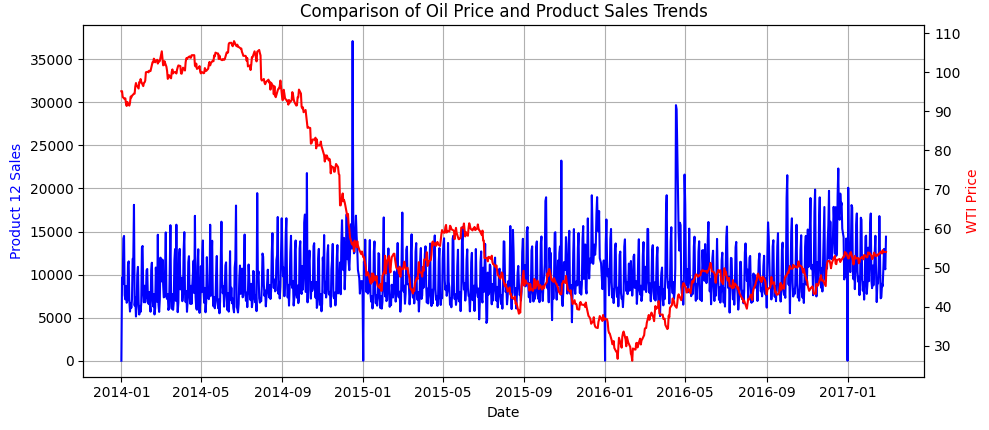
휘발유 가격과 상품 판매량 추이 비교

시계열 패턴 2

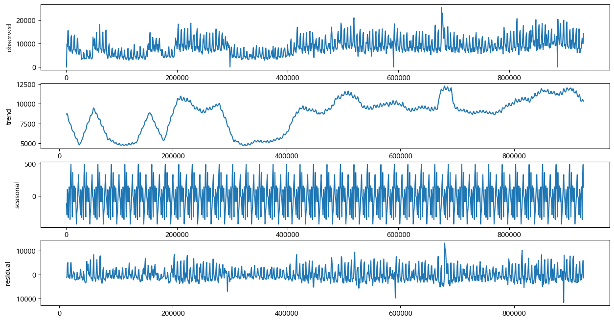
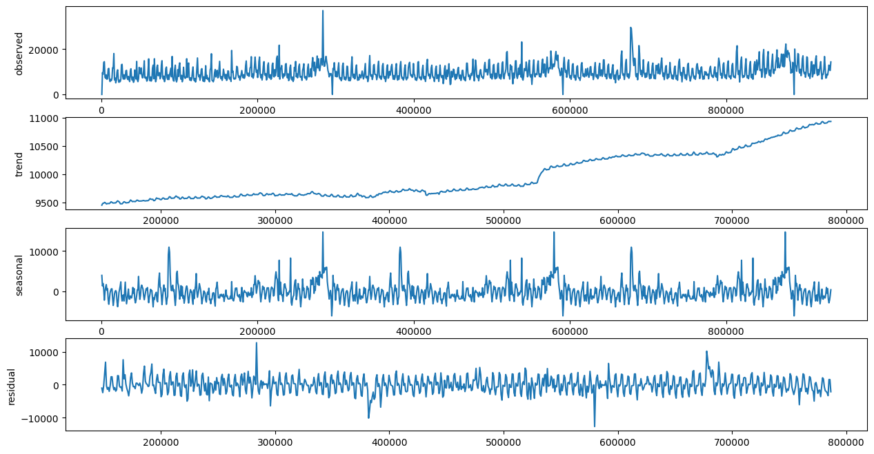
시계열 데이터 분해 (30일 주기)
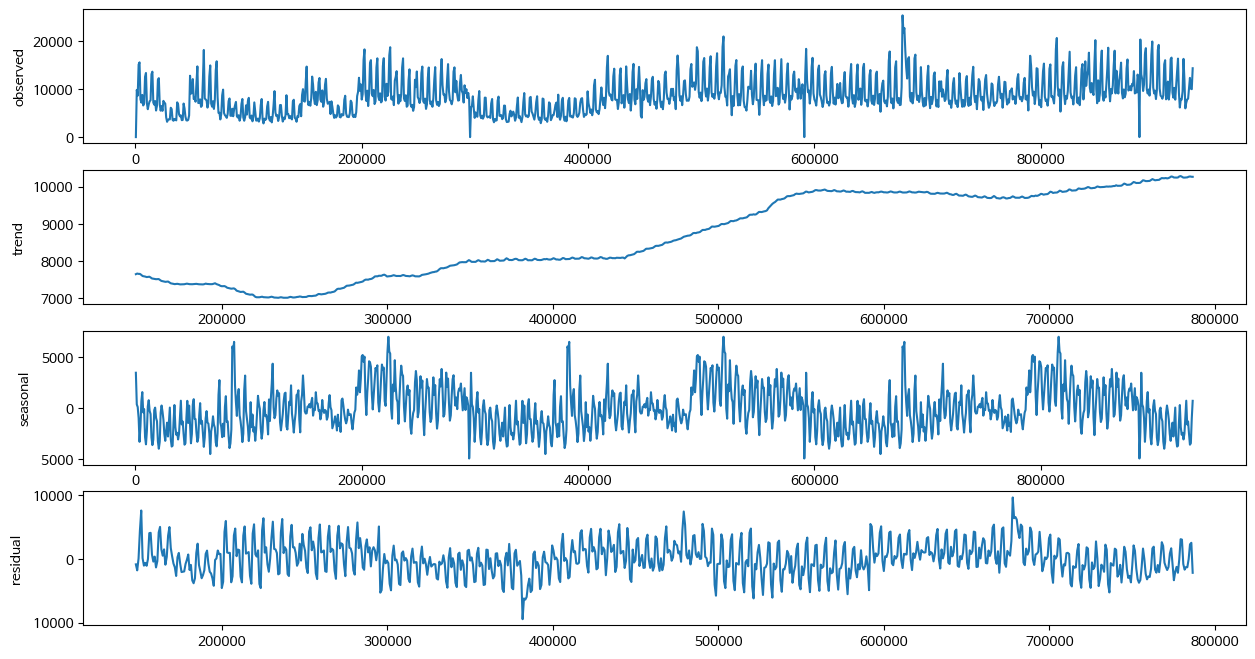
시계열 데이터 분해 (365일 주기)

PRODUCT_ID - 42

시계열 패턴 1

42번 상품의 상품별 판매량 추이
휘발유 가격과 상품 판매량 추이 비교

시계열 패턴 2

시계열 데이터 분해 (30일 주기)
시계열 데이터 분해 (365일 주기)

최종 정리

1) 대상 매장(44), 대상 상품의 판매량 추이

1월에 구매량이 적고, 7월에 구매량이 가장 많음
7월에 구매량이 가장 많은 이유는 5월 ~ 7월에 수확이 이루어지기 때문에 구매가 많을 것으로 예상함
12월에 구매고객수가 제일 많음 => 크리스마스로 인해 가장 많아진 것으로 예상
년도별로 판매량이 증가함

2) 대상 상품의 동일 카테고리의 상품별 판매량 추이

카테고리로 봤을 때, grocery 카테고리는 44번 매장이 가장 많이 팔림
서브카테고리로 봤을 때, 농산물을 파는 곳은 44번 매장 밖에 없었음
44번 매장의 구매고객수는 1주일 주기로 많아짐 => 주로 어떤 것들이 팔리나확인
44번 매장에는 3, 12번 제품이 제일 많이 팔리고, 42번은 그렇게 많이 팔리지 않음

3) 휘발류 가격과 상품 판매량 추이 비교

유가가 비쌀수록 판매량도 감소, 구매고객수는 적게 감소하는 모습을 보임 => 1인당 구매량을 확인해봐야함
판매량 / 구매고객수 = 1인당 구매량을 계산 => 유가가 비쌀수록 1인당 구매량이 적어지는 모습이 보임

4) 입고 시간과 위치, 판매량 추이 비교

입고시간이 길어지면 판매량이 줄 것이다 => 관계는 없었음
입고시간, 도시나 주의 위치와의 관계가 있을까? => 관계 없었음
44번 스토어의 입고 시간이 다른 매장보다 더 길다 => 왜 그렇지??

Product_ID (12)

12번 항목과 휘발류 가격에는 연관성이 없다.
12번 항목의 판매량과 방문 고객 수는 비례한다.
12번 항목은 판매 변화량이 균일하게 유지된다.
수요일, 금요일, 토요일에 판매량이 증가하는 경향이 있고, 화요일, 목요일, 일요일에는 판매량이 감소하는 경향이 있다.
365일 기준으로 봤을때 연도가 지날수록 판매량이 증가하는 추세를 보인다.
미국은 12월 기준으로 유제품 판매량이 급증한다. => 에그노그를 먹는 풍습이 있음
미국의 2014년 01월 ~ 2017년 02월 까지 스타벅스의 주가상승이 있었음 => 그 만큼 유통업체의 판매량이 증가했음 그 이유는 스타벅스에서 판매하는 메뉴는 유제품 사용이 많기 때문이다.

2. 데이터 전처리 및 base_line_modeling

3번의 모델링 및 비즈니스 평가를 위해 기본 레이어층만 쌓아서 수행할 모델을 생성

PRODUCT_ID - 3

DecisionTreeRegressor

MSE : 3549.151657936104
MAE : 2528.9166666666665
MAPE : 0.221088798045424
R2 Score : 0.09131166924273626

딥러닝

MSE : 3549.151657936104
MAE : 2528.9166666666665
MAPE : 0.221088798045424
R2 Score : 0.09131166924273626

LSTM

LSTM 모델은 return_sequence=True 을 사용 => 시계열 모델에서 양방향으로 확인을 하는 것임

clear_session()

model_LSTM = Sequential()

model_LSTM.add(LSTM(128, input_shape = (timesteps, n_features),
                    return_sequences = True))
model_LSTM.add(LSTM(64, return_sequences = True))
model_LSTM.add(LSTM(32, return_sequences = True))
model_LSTM.add(LSTM(16))

model_LSTM.add(Dense(8, activation = 'selu'))
model_LSTM.add(Dense(4, activation = 'selu'))
model_LSTM.add(Dense(1))

model_LSTM.compile(optimizer = Adam(learning_rate = 0.001), loss='mse')
model_LSTM.summary()

PRODUCT_ID - 12

딥러닝

학습 RMSE: 0.06607926449502957
검증 RMSE: 0.05921918568987373
학습 MAE: 0.03685247268320722
검증 MAE: 0.04013581683132576
학습 MAPE: inf
검증 MAPE: inf
학습 R2 점수: 0.5092537047409504
검증 R2 점수: 0.6654690033907339

LSTM

x, y를 분할

x = df_product12_final.drop('target', axis=1)
y = df_product12_final.loc[:, 'target']

2차원에서 3차원으로 변환함

# 하루를 한 단위로 묶겠다
timesteps = 24
x2, y2 = temporalize(x, y, timesteps)

3차원 스케일링

def scale(X, scaler):
    for i in range(X.shape[0]):
        X[i, :, :] = scaler.fit_transform(X[i, :, :])
    return X

# 3차원 스케일링
from sklearn.preprocessing import MinMaxScaler
scaler = MinMaxScaler()

# X_train
X_train_s = scale(X_train, scaler)

# X_val
X_val_s = scale(X_val, scaler)

y 스케일링

# y 스케일링
scaler = MinMaxScaler()

y_train_s = scaler.fit_transform(y_train.reshape(-1,1))
y_val_s = scaler.transform(y_val.reshape(-1,1))

LSTM 적용

from keras.models import Sequential
from keras.layers import LSTM, Dense

model_lstm = Sequential()
model_lstm.add(LSTM(50, input_shape=(X_train_s.shape[1], X_train_s.shape[2])))
model_lstm.add(Dense(1))
model_lstm.compile(optimizer='adam', loss='mse')

print("LSTM 모델 구조")
print(model_lstm.summary())

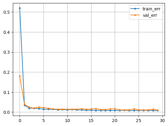
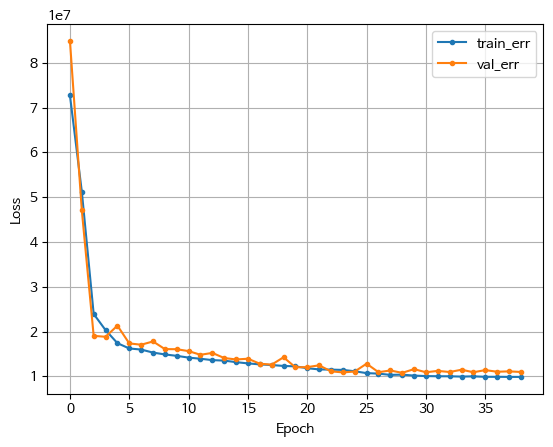
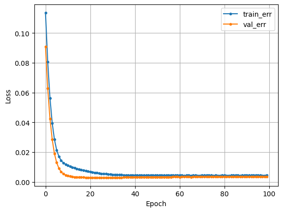
history = model_lstm.fit(X_train_s, y_train_s, epochs=50, validation_split=.2).history

LSTM 시각화

plt.plot(history['loss'], label = 'train_err', marker = '.')
plt.plot(history['val_loss'], label = 'val_err', marker = '.')
plt.grid()
plt.legend()
plt.show()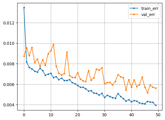

CNN

from keras.models import Sequential
from keras.layers import Conv1D, MaxPooling1D, Flatten, Dense

model_cnn = Sequential()
model_cnn.add(Conv1D(filters=64, kernel_size=3, activation='relu', input_shape=(X_train_s.shape[1], X_train_s.shape[2]), padding = 'same'))
model_cnn.add(MaxPooling1D(pool_size=2))
model_cnn.add(Flatten())
model_cnn.add(Dense(50, activation='relu'))
model_cnn.add(Dense(1))
model_cnn.compile(optimizer='adam', loss='mse')

print("CNN 모델 구조")
print(model_cnn.summary())

history = model_cnn.fit(X_train_s, y_train_s, epochs=50, validation_split=.2).history

시각화

plt.plot(history['loss'], label = 'train_err', marker = '.')
plt.plot(history['val_loss'], label = 'val_err', marker = '.')
plt.grid()
plt.legend()
plt.show()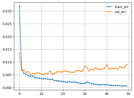

PRODUCT_ID - 42

머신러닝

DecisionTreeRegressor

RMSE 24.635519509689512

MAE 19.186147186147185

RandomForestRegressor

RMSE 18.32681937726738

MAE 14.461006258846675

XGBRegressor

RMSE 19.054946252551975

MAE 14.925340971019674

LGBMRegressor

RMSE 18.8105078934692

MAE 14.729264357818643

LinearRegression

RMSE 35.299717336187015

MAE 29.73039955720623

LSTM

전처리

def flatten(X):
    flattened_X = np.empty((X.shape[0], X.shape[2]))
    for i in range(X.shape[0]):
        flattened_X[i] = X[i, (X.shape[1]-1), :]
    return flattened_X

def scale(X, scaler):
    for i in range(X.shape[0]):
        X[i, :, :] = scaler.transform(X[i, :, :])
    return X

2차원 -> 3차원

# 2차원으로 변환하여 스케일러 생성
scaler = MinMaxScaler().fit(flatten(x_train))

스케일링

# y에 대한 스케일링(최적화를 위해)
scaler_y = MinMaxScaler()
y_train_s3 = scaler_y.fit_transform(y_train.reshape(-1,1))
y_val_s3 = scaler_y.transform(y_val.reshape(-1,1))

LSTM

clear_session()

model = Sequential([LSTM(32, input_shape=(timesteps, n_features), return_sequences=True),
                    LSTM(16,return_sequences=False),
                    Dense(1)])
model.summary()

시각화

plt.plot(hist['loss'], label = 'train_err', marker = '.')
plt.plot(hist['val_loss'], label = 'val_err', marker = '.')
plt.grid()
plt.legend()
plt.show()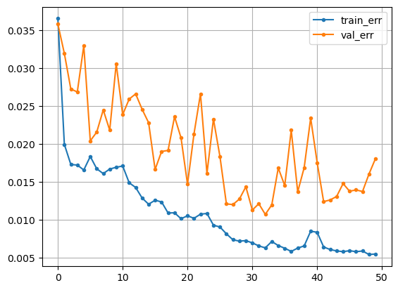

CNN

n_features = x_train.shape[2]

clear_session()

model3 = Sequential([Conv1D(32, 5, input_shape = (timesteps, n_features), activation='relu', padding = 'same'),
                    Flatten(),
                    Dense(1)])

model3.compile(optimizer= Adam(learning_rate = 0.01) ,loss='mse')

시각화

plt.plot(hist['loss'], label = 'train_err', marker = '.')
plt.plot(hist['val_loss'], label = 'val_err', marker = '.')
plt.grid()
plt.legend()
plt.show()

정지원

뒤늦게 프로그래밍을 시작한 응애

이전 포스트

10주차 5차 미니프로젝트

다음 포스트

10주차 6차 미니프로젝트 (1차)

에이블 스쿨 복습

1. 데이터 탐색 및 가설 도출

PRODUCT_ID - 3

시계열 패턴 1

시계열 패턴 2

PRODUCT_ID - 12

시계열 패턴 1

시계열 패턴 2

PRODUCT_ID - 42

시계열 패턴 1

시계열 패턴 2

최종 정리

1) 대상 매장(44), 대상 상품의 판매량 추이

2) 대상 상품의 동일 카테고리의 상품별 판매량 추이

3) 휘발류 가격과 상품 판매량 추이 비교

4) 입고 시간과 위치, 판매량 추이 비교

Product_ID (12)

2. 데이터 전처리 및 base_line_modeling

PRODUCT_ID - 3

DecisionTreeRegressor

딥러닝

LSTM

PRODUCT_ID - 12

딥러닝

LSTM

CNN

PRODUCT_ID - 42

머신러닝

LSTM

CNN

10주차 5차 미니프로젝트

11주차 6차 미니프로젝트 (2차)

0개의 댓글