Baseline 모델 (1) 라이브러리, 데이터 가져오기
실제 Baseline 커널에 있는 내용을 참고하여 코드를 작성해 봅시다.
import warnings
warnings.filterwarnings("ignore")

import os
from os.path import join

import pandas as pd
import numpy as np

import missingno as msno

from sklearn.ensemble import GradientBoostingRegressor
from sklearn.model_selection import KFold, cross_val_score
import xgboost as xgb
import lightgbm as lgb

import matplotlib.pyplot as plt
%matplotlib inline
%config InlineBackend.figure_format = 'retina'
import seaborn as sns
# 데이터 경로 수정
data_dir = os.getenv('HOME')+'/aiffel/kaggle_kakr_housing/data'
train_data_path = join(data_dir, 'train.csv')
sub_data_path = join(data_dir, 'test.csv') Baseline 모델 (2) 데이터 이해하기
1. 데이터 살펴보기
pandas의 read_csv 함수를 사용해 데이터를 읽어오고, 각 변수들이 나타내는 의미를 살펴보겠습니다.
이 특징들을 이용하여 집의 가격을 예측해야 합니다.
- ID : 집을 구분하는 번호
- date : 집을 구매한 날짜
- price : 타겟 변수인 집의 가격
- bedrooms : 침실의 수
- bathrooms : 침실당 화장실 개수
- sqft_living : 주거 공간의 평방 피트
- sqft_lot : 부지의 평방 피트
- floors : 집의 층 수
- waterfront : 집의 전방에 강이 흐르는지 유무 (a.k.a. 리버뷰)
- view : 집이 얼마나 좋아 보이는지의 정도
- condition : 집의 전반적인 상태
- grade : King County grading 시스템 기준으로 매긴 집의 등급
- sqft_above : 지하실을 제외한 평방 피트
- sqft_basement : 지하실의 평방 피트
- yr_built : 집을 지은 년도
- yr_renovated : 집을 재건축한 년도
- zipcode : 우편번호
- lat : 위도
- long : 경도
- sqft_living15 : 2015년 기준 주거 공간의 평방 피트(집을 재건축했다면, 변화가 있을 수 있음)
- sqft_lot15 : 2015년 기준 부지의 평방 피트(집을 재건축했다면, 변화가 있을 수 있음)
# ✓ 데이터 불러오기
# 데이터를 data, sub이라는 변수로 불러옵니다.

data = pd.read_csv(train_data_path)
sub = pd.read_csv(sub_data_path)
print('train data dim : {}'.format(data.shape))
print('sub data dim : {}'.format(sub.shape))
train data dim : (15035, 21)
sub data dim : (6468, 20)# ✓ 학습 데이터에서 라벨 제거하기
# price 컬럼을 y라는 변수에 저장한 후 해당 컬럼은 지워줍니다.
y = data['price']
del data['price']
print(data.columns)Index(['id', 'date', 'bedrooms', 'bathrooms', 'sqft_living', 'sqft_lot',
'floors', 'waterfront', 'view', 'condition', 'grade', 'sqft_above',
'sqft_basement', 'yr_built', 'yr_renovated', 'zipcode', 'lat', 'long',
'sqft_living15', 'sqft_lot15'],
dtype='object')# ✓ 학습 데이터와 테스트 데이터 합치기
# 모델 학습 전, 전체 데이터를 보기 위해 합쳐봅시다.(물론 모델 학습을 진행할 때 다시 분리해서 사용해줘야 합니다.)
train_len = len(data) # 나중에 분리하기 위해 train데이터의 인덱스로써 저장시킵니다.
data = pd.concat((data, sub), axis=0)data.head()| id | date | bedrooms | bathrooms | sqft_living | sqft_lot | floors | waterfront | view | condition | grade | sqft_above | sqft_basement | yr_built | yr_renovated | zipcode | lat | long | sqft_living15 | sqft_lot15 | |
|---|---|---|---|---|---|---|---|---|---|---|---|---|---|---|---|---|---|---|---|---|
| 0 | 0 | 20141013T000000 | 3 | 1.00 | 1180 | 5650 | 1.0 | 0 | 0 | 3 | 7 | 1180 | 0 | 1955 | 0 | 98178 | 47.5112 | -122.257 | 1340 | 5650 |
| 1 | 1 | 20150225T000000 | 2 | 1.00 | 770 | 10000 | 1.0 | 0 | 0 | 3 | 6 | 770 | 0 | 1933 | 0 | 98028 | 47.7379 | -122.233 | 2720 | 8062 |
| 2 | 2 | 20150218T000000 | 3 | 2.00 | 1680 | 8080 | 1.0 | 0 | 0 | 3 | 8 | 1680 | 0 | 1987 | 0 | 98074 | 47.6168 | -122.045 | 1800 | 7503 |
| 3 | 3 | 20140627T000000 | 3 | 2.25 | 1715 | 6819 | 2.0 | 0 | 0 | 3 | 7 | 1715 | 0 | 1995 | 0 | 98003 | 47.3097 | -122.327 | 2238 | 6819 |
| 4 | 4 | 20150115T000000 | 3 | 1.50 | 1060 | 9711 | 1.0 | 0 | 0 | 3 | 7 | 1060 | 0 | 1963 | 0 | 98198 | 47.4095 | -122.315 | 1650 | 9711 |
2. 간단한 전처리
각 변수들에 대해 결측 유무를 확인하고, 분포를 확인해보면서 간단하게 전처리를 하겠습니다.
✓ 결측치 확인
먼저 데이터에 결측치가 있는지를 확인하겠습니다.
missingno 라이브러리의 matrix 함수를 사용하면, 데이터의 결측 상태를 시각화를 통해 살펴볼 수 있습니다.
msno.matrix(data)<AxesSubplot:>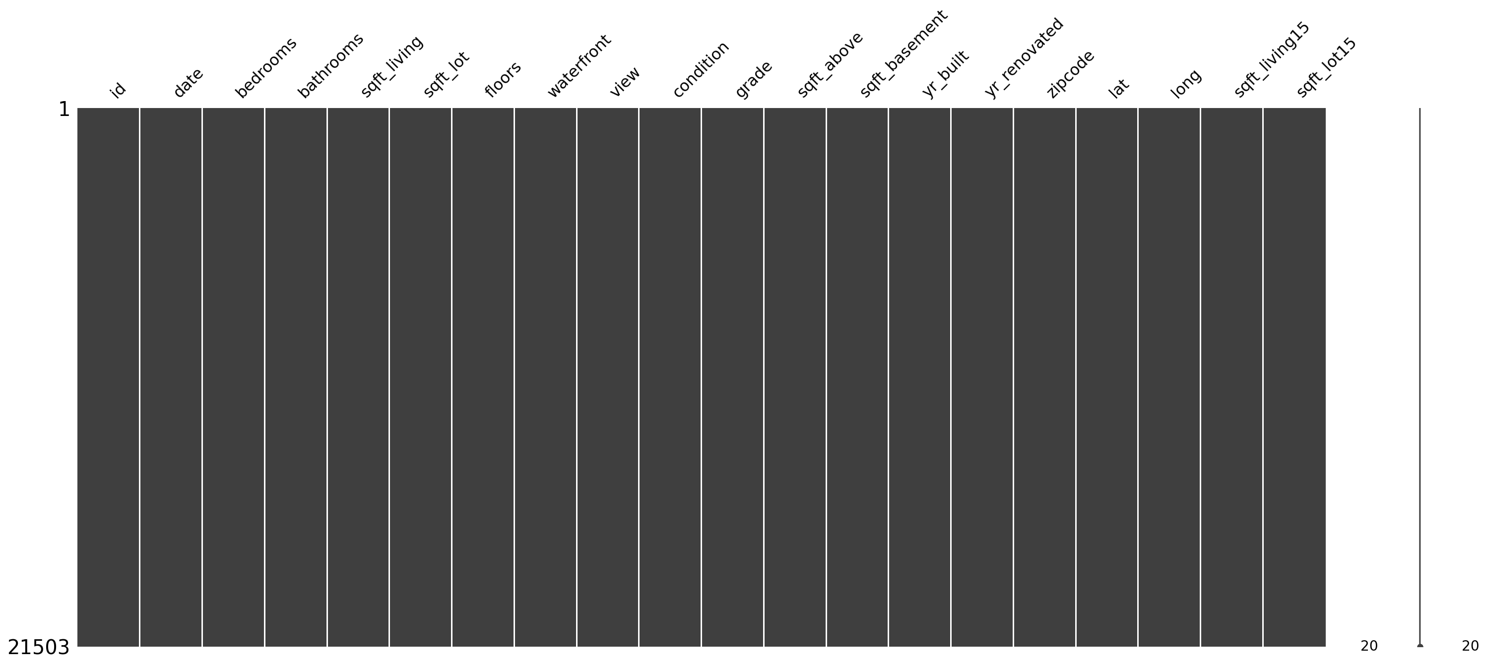
모든 변수에 결측치가 없는 것으로 보이지만, 혹시 모르니 확실하게 살펴보겠습니다.
for c in data.columns:
    print('{} : {}'.format(c, len(data.loc[pd.isnull(data[c]), c].values)))
id : 0
date : 0
bedrooms : 0
bathrooms : 0
sqft_living : 0
sqft_lot : 0
floors : 0
waterfront : 0
view : 0
condition : 0
grade : 0
sqft_above : 0
sqft_basement : 0
yr_built : 0
yr_renovated : 0
zipcode : 0
lat : 0
long : 0
sqft_living15 : 0
sqft_lot15 : 0- 인덱싱을 사용하면, 데이터프레임을 이용해서 데이터프레임으로부터 원하는 값을 가져올 수 있습니다다!!
- 인덱싱을 이용하면 데이터프레임을 그대로 사용할 수 있다는 것이 매우 큰 장점이다. 인덱싱 기능이 없다면 항상 데이터프레임을 배열로 바꾸고 for문을 사용해야 합니다.
- 속도면에서도 월등히 빠릅니다.
✓ id, date 변수 정리
id 변수는 모델이 집값을 예측하는데 도움을 주지 않으므로 제거합니다.
date 변수는 연월일시간으로 값을 가지고 있는데, 연월만 고려하는 범주형 변수로 만들겠습니다.
추후 예측 결과를 제출할 때를 대비하여, sub_id변수에 id칼럼을 저장해두고 지워주도록 합니다.
data 컬럼은 apply함수로 필요한 부분만 잘라줍니다.
sub_id = data['id'][train_len:]
del data['id']
data['date'] = data['date'].apply(lambda x : str(x[:6])).astype(str)
✓ 각 변수들의 분포 확인
한쪽으로 치우친 분포는 모델이 결과를 예측하기에 좋지 않은 영향을 미치므로 다듬어줄 필요가 있습니다.
fig, ax = plt.subplots(9, 2, figsize=(12, 50))   # 가로스크롤 때문에 그래프 확인이 불편하다면 figsize의 x값을 조절해 보세요.

# id 변수(count==0인 경우)는 제외하고 분포를 확인합니다.
count = 1
columns = data.columns
for row in range(9):
    for col in range(2):
        sns.kdeplot(data=data[columns[count]], ax=ax[row][col])
        ax[row][col].set_title(columns[count], fontsize=15)
        count += 1
        if count == 19 :
            break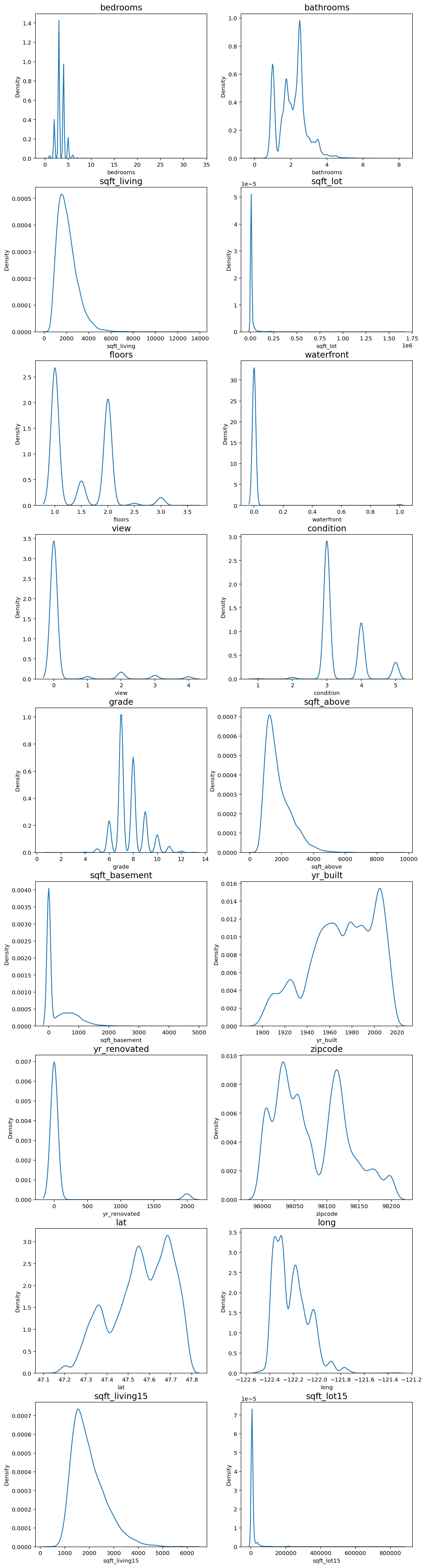
price, bedrooms, sqft_living, sqft_lot, sqft_above, sqft_basement 변수가 한쪽으로 치우친 경향을 보였습니다.
log-scaling을 통해 데이터 분포를 정규분포에 가깝게 만들어 보겠습니다.
skew_columns = ['bedrooms', 'sqft_living', 'sqft_lot', 'sqft_above', 'sqft_basement', 'sqft_lot15', 'sqft_living15']

for c in skew_columns:
    data[c] = np.log1p(data[c].values)

print('얍💢')얍💢fig, ax = plt.subplots(4, 2, figsize=(12, 24))
count = 0
for row in range(4):
for col in range(2):
if count == 7:
break
sns.kdeplot(data=data[skew_columns[count]], ax=ax[row][col])
ax[row][col].set_title(skew_columns[count], fontsize=15)
count += 1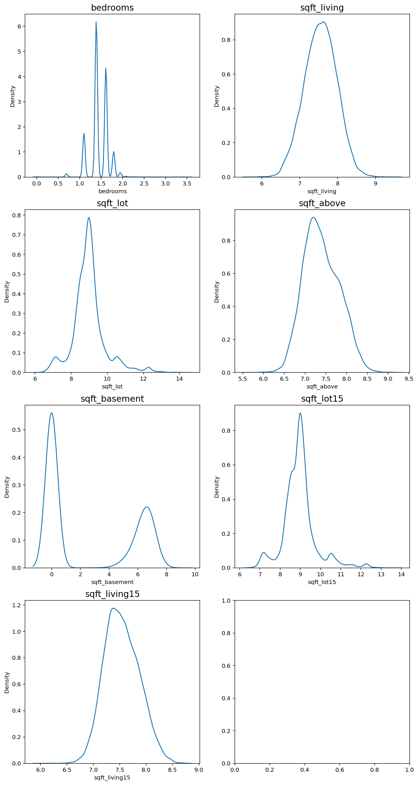
어느정도 치우침이 줄어든 분포를 확인할 수 있습니다.
sub = data.iloc[train_len:, :]
x = data.iloc[:train_len, :]
3. 모델링
- 앙상블 학습: 여러 개의 학습 알고리즘을 사용하고, 그 예측을 결합하여 보다 정확한 최종 예측을 도출한다.
- voting: 여러 모델이 분류해 낸 결과들로부터 다수결 투표로 최종 결과를 선택하는 방법. 분류 문제에서 사용
- averaging: 각 모델이 계산해 낸 실숫값들을 평균 혹은 가중평균하여 사용하는 방법. 회귀 문제에서 사용
✓ Average Blending
여러가지 모델의 결과를 산술 평균을 통해 Blending 모델을 만들겠습니다. 블렌딩이란 하나의 개별 모델을 사용하는 것이 아니라 다양한 여러 모델을 종합하여 결과를 얻는 기법입니다.
gboost = GradientBoostingRegressor(random_state=2019)
xgboost = xgb.XGBRegressor(random_state=2019)
lightgbm = lgb.LGBMRegressor(random_state=2019)

models = [{'model':gboost, 'name':'GradientBoosting'}, {'model':xgboost, 'name':'XGBoost'},
          {'model':lightgbm, 'name':'LightGBM'}]

print('얍💢')얍💢✓ Cross Validation
교차 검증을 통해 모델의 성능을 간단히 평가하겠습니다.
def get_cv_score(models):
    kfold = KFold(n_splits=5).get_n_splits(x.values)
    for m in models:
        CV_score = np.mean(cross_val_score(m['model'], X=x.values, y=y, cv=kfold))
        print(f"Model: {m['name']}, CV score:{CV_score:.4f}")
print('얍💢')얍💢get_cv_score(models)Model: GradientBoosting, CV score:0.8598
Model: XGBoost, CV score:0.8860
Model: LightGBM, CV score:0.8819✓ Make Submission
회귀 모델의 경우에는 cross_val_score 함수가 R2를 반환합니다.
R2 값이 1에 가까울수록 모델이 데이터를 잘 표현함을 나타냅니다.
3개 트리 모델이 상당히 훈련 데이터에 대해 괜찮은 성능을 보여주고 있습니다. Baseline 모델에서는 여러 모델을 입력하면 각 모델에 대한 예측 결과를 평균 내어주는 AveragingBleding()함수를 만들어 사용합니다. 이 함수는 models 딕셔너리 안에 있는 모델을 모두 x,y로 학습시킨 뒤 predictions에 그 예측 결괏값을 모아서 평균한 값을 반환합니다.
훈련 데이터셋으로 3개 모델을 학습시키고, Average Blending을 통해 제출 결과를 만들겠습니다.
def AveragingBlending(models, x, y, sub_x):
    for m in models :
        m['model'].fit(x.values, y)

    predictions = np.column_stack([
        m['model'].predict(sub_x.values) for m in models
    ])
    return np.mean(predictions, axis=1)

print('얍💢')얍💢# 함수를 활용해 예측값을 생성
y_pred = AveragingBlending(models, x, y, sub)
print(len(y_pred))
y_pred6468
array([ 529966.66304912, 430726.21272617, 1361676.91242777, ...,
452081.69137012, 341572.97685942, 421725.1231835 ])# 캐글에 제출하기 위한 csv파일을 확인하기 by lms
data_dir = os.getenv('HOME')+'/aiffel/kaggle_kakr_housing/data'
submission_path = join(data_dir, 'sample_submission.csv')
submission = pd.read_csv(submission_path)
submission.head()| id | price | |
|---|---|---|
| 0 | 15035 | 100000 |
| 1 | 15036 | 100000 |
| 2 | 15037 | 100000 |
| 3 | 15038 | 100000 |
| 4 | 15039 | 100000 |
#id,price로 구성된 데이터 프레임
result = pd.DataFrame({
    'id' : sub_id,
    'price' : y_pred
})

result.head()| id | price | |
|---|---|---|
| 0 | 15035 | 5.299667e+05 |
| 1 | 15036 | 4.307262e+05 |
| 2 | 15037 | 1.361677e+06 |
| 3 | 15038 | 3.338036e+05 |
| 4 | 15039 | 3.089006e+05 |
#제출하기
my_submission_path = join(data_dir, 'submission.csv')
result.to_csv(my_submission_path, index=False)

print(my_submission_path)/aiffel/aiffel/kaggle_kakr_housing/data/submission.csvsub = pd.DataFrame(data={'id':sub_id,'price':y_pred})sub.to_csv('submission.csv', index=False)랭킹을 올리고 싶다면? (1) 다시 한 번, 내 입맛대로 데이터 준비하기
최적의 모델을 찾아서, 하이퍼 파라미터 튜닝
이제 더 좋은 결과를 얻으려면 어떻게 해야할까? 우리는 아직 모델을 건드려보지 않았다. 이번 스텝에서는 여러 하이퍼 파라미터를 튜닝해보면서 모델의 성능을 끌어올려 볼 것이다.
- 모델 파라미터: 모델이 학습을 하며 최적화되는, 최적화되어야 하는 파라미터
- ex. 선형 회귀의 경우 y_pred = Wx + b로 예측값을 만들어낼 수 있을텐데, 여기서 모델 파라미터는 W이다.
- 하이퍼 파라미터: 모델의 학습을 위해 사전에 사람이 직접 입력해주는 파라미터. 모델학습 과정에서 변하지 않는다.
다시 한번, 내 입맛대로 데이터 준비하기
이제는 주도적으로 데이터를 다뤄보자.
다시 데이터를 가져오는 것부터 시작하자.
data_dir = os.getenv('HOME')+'/aiffel/kaggle_kakr_housing/data'

train_data_path = join(data_dir, 'train.csv')
test_data_path = join(data_dir, 'test.csv')

train = pd.read_csv(train_data_path)
test = pd.read_csv(test_data_path)

print('얍💢')얍💢# 시작 전에 데이터 살펴보기
train.head()| id | date | price | bedrooms | bathrooms | sqft_living | sqft_lot | floors | waterfront | view | ... | grade | sqft_above | sqft_basement | yr_built | yr_renovated | zipcode | lat | long | sqft_living15 | sqft_lot15 | |
|---|---|---|---|---|---|---|---|---|---|---|---|---|---|---|---|---|---|---|---|---|---|
| 0 | 0 | 20141013T000000 | 221900.0 | 3 | 1.00 | 1180 | 5650 | 1.0 | 0 | 0 | ... | 7 | 1180 | 0 | 1955 | 0 | 98178 | 47.5112 | -122.257 | 1340 | 5650 |
| 1 | 1 | 20150225T000000 | 180000.0 | 2 | 1.00 | 770 | 10000 | 1.0 | 0 | 0 | ... | 6 | 770 | 0 | 1933 | 0 | 98028 | 47.7379 | -122.233 | 2720 | 8062 |
| 2 | 2 | 20150218T000000 | 510000.0 | 3 | 2.00 | 1680 | 8080 | 1.0 | 0 | 0 | ... | 8 | 1680 | 0 | 1987 | 0 | 98074 | 47.6168 | -122.045 | 1800 | 7503 |
| 3 | 3 | 20140627T000000 | 257500.0 | 3 | 2.25 | 1715 | 6819 | 2.0 | 0 | 0 | ... | 7 | 1715 | 0 | 1995 | 0 | 98003 | 47.3097 | -122.327 | 2238 | 6819 |
| 4 | 4 | 20150115T000000 | 291850.0 | 3 | 1.50 | 1060 | 9711 | 1.0 | 0 | 0 | ... | 7 | 1060 | 0 | 1963 | 0 | 98198 | 47.4095 | -122.315 | 1650 | 9711 |
5 rows × 21 columns
date를 전처리해주자. Baseline 커널이 했던 것과 달리, 정수형 데이터로 처리해보자!
이렇게 하면 모델이 date도 예측을 위한 특성으로 활용할 수 있을 것이다.
train['date'] = train['date'].apply(lambda i: i[:6]).astype(int)
train.head()| id | date | price | bedrooms | bathrooms | sqft_living | sqft_lot | floors | waterfront | view | ... | grade | sqft_above | sqft_basement | yr_built | yr_renovated | zipcode | lat | long | sqft_living15 | sqft_lot15 | |
|---|---|---|---|---|---|---|---|---|---|---|---|---|---|---|---|---|---|---|---|---|---|
| 0 | 0 | 201410 | 221900.0 | 3 | 1.00 | 1180 | 5650 | 1.0 | 0 | 0 | ... | 7 | 1180 | 0 | 1955 | 0 | 98178 | 47.5112 | -122.257 | 1340 | 5650 |
| 1 | 1 | 201502 | 180000.0 | 2 | 1.00 | 770 | 10000 | 1.0 | 0 | 0 | ... | 6 | 770 | 0 | 1933 | 0 | 98028 | 47.7379 | -122.233 | 2720 | 8062 |
| 2 | 2 | 201502 | 510000.0 | 3 | 2.00 | 1680 | 8080 | 1.0 | 0 | 0 | ... | 8 | 1680 | 0 | 1987 | 0 | 98074 | 47.6168 | -122.045 | 1800 | 7503 |
| 3 | 3 | 201406 | 257500.0 | 3 | 2.25 | 1715 | 6819 | 2.0 | 0 | 0 | ... | 7 | 1715 | 0 | 1995 | 0 | 98003 | 47.3097 | -122.327 | 2238 | 6819 |
| 4 | 4 | 201501 | 291850.0 | 3 | 1.50 | 1060 | 9711 | 1.0 | 0 | 0 | ... | 7 | 1060 | 0 | 1963 | 0 | 98198 | 47.4095 | -122.315 | 1650 | 9711 |
5 rows × 21 columns
두 번째로 할 일은 타겟 데이터 price 컬럼을 y 변수에 넣어두고 train data에서는 삭제하는 것이다.
y = train['price']
del train['price']
id 컬럼까지 삭제해주면 기본적인 전처리는 마무리된다.
del train['id']

print(train.columns)
Index(['date', 'bedrooms', 'bathrooms', 'sqft_living', 'sqft_lot', 'floors',
'waterfront', 'view', 'condition', 'grade', 'sqft_above',
'sqft_basement', 'yr_built', 'yr_renovated', 'zipcode', 'lat', 'long',
'sqft_living15', 'sqft_lot15'],
dtype='object')test data에 대해서도 동일한 작업을 진행해준다. 단, test에 우리가 맞추어야 할 타겟 데이터인 price는 없으니, 훈련 데이터셋과는 다르게 price에 대한 처리는 필요없다.
# test의 id 컬럼 삭제
test['date'] = test['date'].apply(lambda i: i[:6]).astype(int)

del test['id']

print(test.columns)
Index(['date', 'bedrooms', 'bathrooms', 'sqft_living', 'sqft_lot', 'floors',
'waterfront', 'view', 'condition', 'grade', 'sqft_above',
'sqft_basement', 'yr_built', 'yr_renovated', 'zipcode', 'lat', 'long',
'sqft_living15', 'sqft_lot15'],
dtype='object')# target data인 y 살펴보기
y0 221900.0
1 180000.0
2 510000.0
3 257500.0
4 291850.0
...
15030 610685.0
15031 1007500.0
15032 360000.0
15033 400000.0
15034 325000.0
Name: price, Length: 15035, dtype: float64# seaborn의 kdeplot을 활용해 y의 분포를 확인하기
sns.kdeplot(y)
plt.show()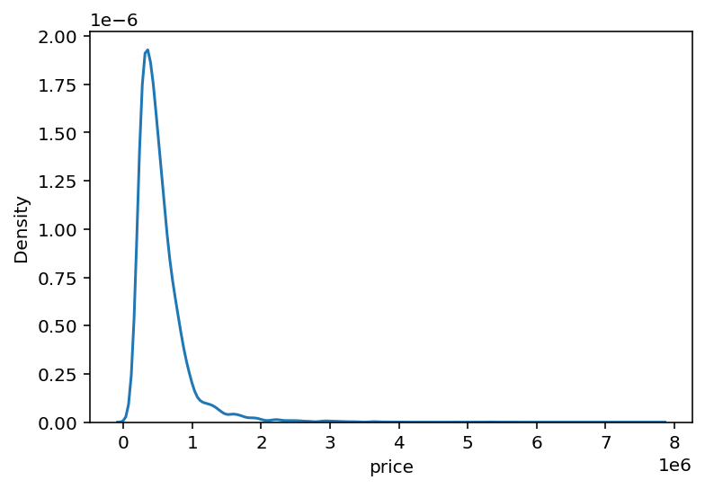
앞서 살펴봤듯이, 왼쪽으로 크게 치우쳐져 있는 형태이다. 따라서 y는 np.log1p()함수를 통해 로그 벼환을 하고, 나중에 모델이 값을 예측한 후에 다시 np.expm1()을 활용해서 되돌려주자.(np.expm1(): 각 원소 x마다 exp(x)-1의 값을 반환해준다.)
y = np.log1p(y)
y
0 12.309987
1 12.100718
2 13.142168
3 12.458779
4 12.583999
...
15030 13.322338
15031 13.822984
15032 12.793862
15033 12.899222
15034 12.691584
Name: price, Length: 15035, dtype: float64sns.kdeplot(y)
plt.show()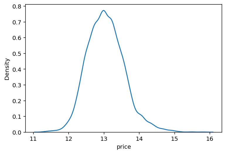
완만한 정규분포의 형태로 변환되었다. dlwp info()함수로 전체 데이터의 자료형을 한눈에 확인해보자.
train.info()<class 'pandas.core.frame.DataFrame'>
RangeIndex: 15035 entries, 0 to 15034
Data columns (total 19 columns):
# Column Non-Null Count Dtype
--- ------ -------------- -----
0 date 15035 non-null int64
1 bedrooms 15035 non-null int64
2 bathrooms 15035 non-null float64
3 sqft_living 15035 non-null int64
4 sqft_lot 15035 non-null int64
5 floors 15035 non-null float64
6 waterfront 15035 non-null int64
7 view 15035 non-null int64
8 condition 15035 non-null int64
9 grade 15035 non-null int64
10 sqft_above 15035 non-null int64
11 sqft_basement 15035 non-null int64
12 yr_built 15035 non-null int64
13 yr_renovated 15035 non-null int64
14 zipcode 15035 non-null int64
15 lat 15035 non-null float64
16 long 15035 non-null float64
17 sqft_living15 15035 non-null int64
18 sqft_lot15 15035 non-null int64
dtypes: float64(4), int64(15)
memory usage: 2.2 MB랭킹을 올리고 싶다면? (2) 다양한 실험을 위해 함수로 만들어 쓰자
본격적인 모델 튜닝을 해보자. 보다 다양한 실험을 하기 위해서는, 실험을 위한 도구들이 잘 준비되어 있는 것이 유리하다.
따라서 여러 번 반복되는 작업들은 함수로 만들어두고 실험을 하는 것이 좋다.
from sklearn.model_selection import train_test_split
from sklearn.metrics import mean_squared_error

print('얍💢')얍💢✔ RMSE 계산
대회 평가 척도이기 때문에 RMSE를 만들어두자.
주의할 점은, y_test나 y_pred는 위에서 np.log1p()로 변환되었으므로 원래 데이터 단위에 맞게 np.expm1()을 추가해야하 한다.
exp로 변환해서 mean_squred_error를 계산하고, np.sqrt()를 취하면 RMSE가 나올 것이다.
def rmse(y_test, y_pred):
    return np.sqrt(mean_squared_error(np.expm1(y_test), np.expm1(y_pred)))

print('얍💢')얍💢XGBRegressor, LGBMRegressor, GradientBoostingRegressor, RandomForestRegressor 모델을 가져오자
from xgboost import XGBRegressor
from lightgbm import LGBMRegressor
from sklearn.ensemble import GradientBoostingRegressor, RandomForestRegressor

print('얍💢')얍💢모델 인스턴스를 생성하고 models라는 리스트에 넣어주자.
이때, 파라미터 초기화나 데이터셋 구성에 사용되는 랜덤 시드값인 random_state값을 특정 값으로 고정시키거나, None으로 세팅할 수 있다. none으로 지정하면, 모델 내부에서 랜덤 시드값을 임의로 선택하기 때문에, 결과적으로 파라미터 초기화나 데이터셋 구성 양상이 달라져서 모델과 데이터셋이 동일하더라도 머신러닝 학습결과는 학습할 때마다 달라진다.
앞으로는 베이스라인에서 시작해서 여러 실험을 통해 성능이 개선되는지를 검증해보자. 이떄, 어떤 시도가 모델 성능 향상에 긍정적인지 부정적인지 여부를 판단하기 위해서는 랜덤적 요소의 변화 때문에 생기는 불확실성을 제거해야 한다. 따라서, random_state 값을 고정시킬 것이다.
# random_state는 모델초기화나 데이터셋 구성에 사용되는 랜덤 시드값입니다.
#random_state=None    # 이게 초기값입니다. 아무것도 지정하지 않고 None을 넘겨주면 모델 내부에서 임의로 선택합니다.
random_state=2020        # 하지만 우리는 이렇게 고정값을 세팅해 두겠습니다.

gboost = GradientBoostingRegressor(random_state=random_state)
xgboost = XGBRegressor(random_state=random_state)
lightgbm = LGBMRegressor(random_state=random_state)
rdforest = RandomForestRegressor(random_state=random_state)

models = [gboost, xgboost, lightgbm, rdforest]

print('얍💢')얍💢gboost.__class__.__name__ #모델명은 클래스의 __name__속성세 접근해서 얻는다.'GradientBoostingRegressor'# 이름을 접근할 수 있기 때문에, for문 내에서 모델별로 학습/예측이 가능하다.
df = {}
for model in models:
# 모델 이름 획득
model_name = model.__class__.__name__
# train, test 데이터셋 분리 - 여기에도 random_state를 고정합니다.
X_train, X_test, y_train, y_test = train_test_split(train, y, random_state=random_state, test_size=0.2)
# 모델 학습
model.fit(X_train, y_train)
# 예측
y_pred = model.predict(X_test)
# 예측 결과의 rmse값 저장
df[model_name] = rmse(y_test, y_pred)
# data frame에 저장
score_df = pd.DataFrame(df, index=['RMSE']).T.sort_values('RMSE', ascending=False)
df{'GradientBoostingRegressor': 128360.19649691365,
'XGBRegressor': 110318.66956616656,
'LGBMRegressor': 111920.36735892233,
'RandomForestRegressor': 125487.07102453562}이렇게 네 모델에 대해 RMSE값을 얻을 수 있었다.
위 과정을 get_scores(models, train, y) 함수로 만들어보자.
def get_scores(models, train, y):
    # 답안 작성
    df = {}
    for model in models:
        model_name = model.__class__.__name__

        # train test split
        X_train, X_test, y_train, y_test = train_test_split(train, y, random_state=random_state, test_size=0.2)

        # 모델 학습
        model.fit(X_train, y_train)

        # 예측
        y_pred = model.predict(X_test)

        # 예측 결과의 rmse값 저장
        df[model_name] = rmse(y_test, y_pred)

        # df
        score_df = pd.DataFrame(df, index=['RMSE']).T.sort_values("RMSE", ascending=False)
    return score_df

get_scores(models, train, y)| RMSE | |
|---|---|
| GradientBoostingRegressor | 128360.196497 |
| RandomForestRegressor | 125487.071025 |
| LGBMRegressor | 111920.367359 |
| XGBRegressor | 110318.669566 |
랭킹을 올리고 싶다면? (3) 하이퍼 파라미터 튜닝의 최강자, 그리드 탐색
모델과 데이터셋이 있다면 RMSE 결괏값을 나타내주는 함수가 준비되었으니, 여러 하이퍼 파라미터로 실험해보자.
실험은 sklearn.model_selection라이브러리 안에 있는 GridSearchCV클래스를 사용한다. GridSearCV는 다양한 파라미터를 입력하면 가능한 모든 조합을 탐색해준다.
from sklearn.model_selection import GridSearchCV


print('얍💢')얍💢GridSearchCV란 무엇인지 알기 전에, 그리드 탐색과 랜덤 탐색을 알아보자. 두 가지 모두 하이퍼 파라미터를 조합해보는 방법이다.
-
그리드 탐색: 사람이 먼저 탐색할 하이퍼 파라미터 값을 정해두고, 그 값들로 만들어질 수 있는 모든 조합을 탐색하는 방법
- 특정 값에 대한 하이퍼 파라미터 조합을 모두 탐색하고자 할 때 유리하다.
- 사람이 정한 값에서만 탐색하기 때문에 최적의 조합을 놓칠 수도 있다.
-
랜덤 탐색: 사람이 탐색할 하이퍼 파라미터의 공간만 정해주고, 그 안에서 랜덤으로 조합을 선택해 탐색하는 방법
- 랜덤으로 탐색하기 때문에 최적의 조합을 찾을 가능성이 있다.
[Bergstra, J., Bengio, Y.: Random search for hyper-parameter optimization. Journal of Machine Learning Research 13, 281–305 (2012), 다음의 블로그에서 재인용]
GridSearchCV에 입력되는 인자들은 다음과 같다.
param_grid: 탐색 파라미터의 종류scoring: 모델 성능을 평가할 지표cv: cross validation을 수행하기 위해 train dataset을 나누는 조각 개수verbose: 그리드 탐색을 진행하며 진행과정을 출력해서 보여줄 메세지의 양n_jobs: 그리트 탐색을 진행하면서 사용할 CPU의 수
이제 param_grid에 탐색할 xgboost관련 하이퍼 파라미터를 넣어보자.
# hyper parameter
param_grid = {
    'n_estimators': [50, 100],
    'max_depth': [1, 10],
}
# 모델 준비
model = LGBMRegressor(random_state=random_state)
print('얍💢')얍💢# GridsearchCV 수행
# grid_model 초기화
grid_model = GridSearchCV(model, param_grid=param_grid, \
scoring='neg_mean_squared_error', \
cv=5, verbose=1, n_jobs=5)
# train과 y데이터로 모델학습
grid_model.fit(train, y)Fitting 5 folds for each of 4 candidates, totalling 20 fits
GridSearchCV(cv=5, estimator=LGBMRegressor(random_state=2020), n_jobs=5,
param_grid={'max_depth': [1, 10], 'n_estimators': [50, 100]},
scoring='neg_mean_squared_error', verbose=1)✔ Fitting 5 folds for each of 4 candidates, totalling 20 fits의 의미
param_grid에 n_estimators x max_depth = 2 x 2 = 4가지 조합 가능
또한, cross valdation을 5번 진행
여기서 cross validation을 5번 진행하는 이유는, 각 조합에 대해 한 번만 실험하는 것보다 5번을 진행해 평균을 취하는 것이 일반화 오차를 추정하는 데에 신뢰도가 더 높기 때문이다.
이제 grid_model.fit 함수를 통해 4가지 조합에 대한 실험을 마쳤다.
실험 결과는 다음과 같이 grid_model.cv_results_안에 저장된다.
# 실험결과
grid_model.cv_results_
{'mean_fit_time': array([0.16141419, 0.25202241, 0.36741648, 0.55432301]),
'std_fit_time': array([0.05594794, 0.06094211, 0.1171111 , 0.08311235]),
'mean_score_time': array([0.01275916, 0.01250086, 0.03050566, 0.03242574]),
'std_score_time': array([0.0098182 , 0.0042731 , 0.01760992, 0.01069391]),
'param_max_depth': masked_array(data=[1, 1, 10, 10],
mask=[False, False, False, False],
fill_value='?',
dtype=object),
'param_n_estimators': masked_array(data=[50, 100, 50, 100],
mask=[False, False, False, False],
fill_value='?',
dtype=object),
'params': [{'max_depth': 1, 'n_estimators': 50},
{'max_depth': 1, 'n_estimators': 100},
{'max_depth': 10, 'n_estimators': 50},
{'max_depth': 10, 'n_estimators': 100}],
'split0_test_score': array([-0.0756974 , -0.05555652, -0.02885847, -0.02665428]),
'split1_test_score': array([-0.07666447, -0.057876 , -0.03041465, -0.02795896]),
'split2_test_score': array([-0.07354904, -0.05546079, -0.03068533, -0.02834112]),
'split3_test_score': array([-0.07510863, -0.05582109, -0.02987609, -0.02774809]),
'split4_test_score': array([-0.06595281, -0.05038773, -0.02605217, -0.02443328]),
'mean_test_score': array([-0.07339447, -0.05502043, -0.02917734, -0.02702714]),
'std_test_score': array([0.00385583, 0.00247946, 0.00168295, 0.00141292]),
'rank_test_score': array([4, 3, 2, 1], dtype=int32)}이 중 우리가 원하는 정보는 어떤 파라미터 조합일 때 점수가 어떻게 나오는지이다. 파라미터 조합은 위 딕셔너리 중 params에, 각각의 테스트 점수는 mean_test_score에 저장되어 있다. 이들만 빼내어 살펴보자.
params = grid_model.cv_results_['params']
params
[{'max_depth': 1, 'n_estimators': 50},
{'max_depth': 1, 'n_estimators': 100},
{'max_depth': 10, 'n_estimators': 50},
{'max_depth': 10, 'n_estimators': 100}]score = grid_model.cv_results_['mean_test_score']
scorearray([-0.07339447, -0.05502043, -0.02917734, -0.02702714])# dataFrame으로
results = pd.DataFrame(params)
results["score"] = score # negative_MSE
results| max_depth | n_estimators | score | |
|---|---|---|---|
| 0 | 1 | 50 | -0.073394 |
| 1 | 1 | 100 | -0.055020 |
| 2 | 10 | 50 | -0.029177 |
| 3 | 10 | 100 | -0.027027 |
# add RMSE score
results['RMSE'] = np.sqrt(-1 * results['score'])
results| max_depth | n_estimators | score | RMSE | |
|---|---|---|---|---|
| 0 | 1 | 50 | -0.073394 | 0.270914 |
| 1 | 1 | 100 | -0.055020 | 0.234564 |
| 2 | 10 | 50 | -0.029177 | 0.170814 |
| 3 | 10 | 100 | -0.027027 | 0.164399 |
하지만 이는 위에서 보았던 10만 단위의 RMSE와는 다른 것을 알 수 있다. 왜일까??
그 이유는 price이다. 우리는 price의 분포가 한쪽으로 치우쳐져 있어 log변환을 했었고, RMSE 변환을 위해 np.expm1함수로 원래대로 복원해서 RMSE값을 계산했었다.
하지만 그리드 탐색에서는 np.expm1()으로 변환하지 않았기 때문이다.
따라서, 사실 RMSE column은 사실은 RMSLE인 것이다.(Root Mean Squared Log Error)
그러니 컬럼명을 맞게 재수정해주자.
results = results.rename(columns={'RMSE': 'RMSLE'})
results| max_depth | n_estimators | score | RMSLE | |
|---|---|---|---|---|
| 0 | 1 | 50 | -0.073394 | 0.270914 |
| 1 | 1 | 100 | -0.055020 | 0.234564 |
| 2 | 10 | 50 | -0.029177 | 0.170814 |
| 3 | 10 | 100 | -0.027027 | 0.164399 |
이제 낮은 순서대로 정렬해주자.
results = results.sort_values("RMSLE")
results| max_depth | n_estimators | score | RMSLE | |
|---|---|---|---|---|
| 3 | 10 | 100 | -0.027027 | 0.164399 |
| 2 | 10 | 50 | -0.029177 | 0.170814 |
| 1 | 1 | 100 | -0.055020 | 0.234564 |
| 0 | 1 | 50 | -0.073394 | 0.270914 |
위 과정을 모두 함수로 만들어 앞으로는 간결하게 사용하자.
# `my_GridSearch(model, train, y, param_grid, verbose=2, n_jobs=5)` 함수를 구현


def my_GridSearch(model, train, y, param_grid, verbose=2, n_jobs=5):

    # 1. GridSearchCV 모델로 `model`을 초기화합니다.
    grid_model = GridSearchCV(model, param_grid=param_grid, \
                        scoring='neg_mean_squared_error', \
                        cv=5, verbose=1, n_jobs=5)

    # 2. 모델을 fitting 합니다.
    grid_model.fit(train, y)

    # 3. params, score에 각 조합에 대한 결과를 저장합니다.
    params = grid_model.cv_results_['params']
    score = grid_model.cv_results_['mean_test_score']

    # 4. 데이터 프레임을 생성
    results = pd.DataFrame(params)
    results["score"] = score

    # 5. RMSLE 값을 추가한 후 점수가 높은 순서로 정렬한 `results`를 반환합니다.
    results['RMSLE'] = np.sqrt(-1 * results['score'])

    results = results.sort_values("RMSLE")
    return results
랭킹을 올리고 싶다면? (4) 제출하는 것도, 빠르고 깔끔하게!
실험 준비가 끝났으니 제출을 해보자. 제출 과정도 함수로 만들어 진행하자.
제일 좋은 조합은 max_depth = 10, n_estimators=100이다.
이 모델로 학습을 해서 예측값인 submission.csv 파일을 만들어서 제출하자.
해당 파라미터로 구성한 모델을 준비하고, 학습 후 예측 결과를 생성하자
model = LGBMRegressor(max_depth=10, n_estimators=100, random_state=random_state)
model.fit(train, y)
prediction = model.predict(test)
prediction = np.expm1(prediction)
prediction
array([ 506766.66784595, 479506.10405112, 1345155.15609376, ...,
449515.92243642, 327402.87855805, 426332.71354302])이제 sample_submission.csv 파일을 가져와보자.
data_dir = os.getenv('HOME')+'/aiffel/kaggle_kakr_housing/data'

submission_path = join(data_dir, 'sample_submission.csv')
submission = pd.read_csv(submission_path)
submission.head()| id | price | |
|---|---|---|
| 0 | 15035 | 100000 |
| 1 | 15036 | 100000 |
| 2 | 15037 | 100000 |
| 3 | 15038 | 100000 |
| 4 | 15039 | 100000 |
이제 이 데이터프레임에 모델이 예측한 값을 씌우면 제출 데이터가 완성된다.
submission['price'] = prediction
submission.head()| id | price | |
|---|---|---|
| 0 | 15035 | 5.067667e+05 |
| 1 | 15036 | 4.795061e+05 |
| 2 | 15037 | 1.345155e+06 |
| 3 | 15038 | 3.122579e+05 |
| 4 | 15039 | 3.338645e+05 |
위 데이터를 csv파일로 저장하며, 파일 이름에 모델 종류와 위에서 확인한 RMSLE 값을 넣어주면 파일들이 깔끔하게 정리될 것이다.
submission_csv_path = '{}/submission_{}_RMSLE_{}.csv'.format(data_dir, 'lgbm', '0.164399')
submission.to_csv(submission_csv_path, index=False)
print(submission_csv_path)/aiffel/aiffel/kaggle_kakr_housing/data/submission_lgbm_RMSLE_0.164399.csv이 과정들을 함수로 정리
def save_submission(model, train, y, test, model_name, rmsle=None):
    model.fit(train, y)
    prediction = model.predict(test)
    prediction = np.expm1(prediction)
    data_dir = os.getenv('HOME')+'/aiffel/kaggle_kakr_housing/data'
    submission_path = join(data_dir, 'sample_submission.csv')
    submission = pd.read_csv(submission_path)
    submission['price'] = prediction
    submission_csv_path = '{}/submission_{}_RMSLE_{}.csv'.format(data_dir, model_name, rmsle)
    submission.to_csv(submission_csv_path, index=False)
print('{} saved!'.format(submission_csv_path))save_submission(model, train, y, test, 'lgbm', rmsle='0.0168')/aiffel/aiffel/kaggle_kakr_housing/data/submission_lgbm_RMSLE_0.0168.csv saved!프로젝트: This is your playground! Leaderboard를 정복해 주세요!
모델의 성능을 최대화하기 위해서는 하이퍼 파라미터 튜닝만 있는 것이 아니다. 예를 들면 EDA 과정을 통해 불필요한 피쳐를 골라내어 수정하는 등의 피처 엔지니어링을 진행함으로써 데이터를 정제하는 것이 매우 중요하다.
✓ 시도해볼 수 있는 방법
- 기존에 있는 데이터의 피처를 모델을 보다 잘 표현할 수 있는 형태로 처리하기 (피처 엔지니어링)
- LGBMRegressor, XGBRegressor, RandomForestRegressor 세 가지 이상의 다양한 모델에 대해 하이퍼 파라미터 튜닝하기
- 다양한 하이퍼 파라미터에 대해 그리드 탐색을 시도해서 최적의 조합을 찾아보기
- Baseline 커널에서 활용했던 블렌딩 방법 활용하기
이를 살펴보며 다른 사람들은 어떻게 성능을 올렸는지 공부하는 것도 매우 좋다.
1. 데이터 준비, 전처리
data loading
data_dir = os.getenv('HOME')+'/aiffel/kaggle_kakr_housing/data'

train_data_path = join(data_dir, 'train.csv')
test_data_path = join(data_dir, 'test.csv')

train = pd.read_csv(train_data_path)
test = pd.read_csv(test_data_path)
데이터 분리
# 타켓, id 데이터 삭제 for trianing
# date change
train['date'] = train['date'].apply(lambda i: i[:6]).astype(int)

y = train['price']
del train['price']
del train['id']

# test의 id 컬럼 삭제
test['date'] = test['date'].apply(lambda i: i[:6]).astype(int)

del test['id']

# y log change
y = np.log1p(y)
2. 하이퍼 파라미터 튜닝
✓ 튜닝해볼 수 있는 모델 클래스 인자
대표적으로 튜닝하는 lightgbm 라이브러리 인자는 다음과 같다.
- max_depth : 의사 결정 나무의 깊이, 정수 사용
- learning_rate : 한 스텝에 이동하는 양을 결정하는 파라미터, 보통 0.0001~0.1 사이의 실수 사용
- n_estimators : 사용하는 개별 모델의 개수, 보통 50~100 이상의 정수 사용
- num_leaves : 하나의 LightGBM 트리가 가질 수 있는 최대 잎의 수
- boosting_type : 부스팅 방식, gbdt, rf 등의 문자열 입력
lightgbm, xgboost 파라미터 설명\
분류-lightgbm
lightgbm, xgboost 하이퍼 파라미터 튜닝 등의 키워드로 검색하면 다양한 하이퍼 파라미터 종류를 찾아볼 수 있다.
from sklearn.model_selection import RandomizedSearchCV

def my_RandomSearch(model, train, y, param, n_iter= 5, verbose=1, n_jobs=5):

    # 1. GridSearchCV 모델로 `model`을 초기화합니다.
    random_model = RandomizedSearchCV(model, param_distributions=param, \
                        scoring='neg_mean_squared_error', \
                              n_iter =  n_iter, \
                        cv=10, verbose=1, n_jobs=-1)

    # 2. 모델을 fitting 합니다.
    random_model.fit(train, y)

    # 3. params, score에 각 조합에 대한 결과를 저장합니다.
    params = random_model.cv_results_['params']
    score = random_model.cv_results_['mean_test_score']

    # 4. 데이터 프레임을 생성
    results = pd.DataFrame(params)
    results["score"] = score

    # 5. RMSLE 값을 추가한 후 점수가 높은 순서로 정렬한 `results`를 반환합니다.
    results['RMSLE'] = np.sqrt(-1 * results['score'])

    results = results.sort_values("RMSLE")
    return results
#try after getting score which is lower 110000
param = {
'n_estimators': [int(x) for x in range(370,450,2)],
'max_depth': [int(x) for x in range(8,10)],
}
n_iter = 100
model = LGBMRegressor(random_state=random_state)
my_RandomSearch(model, train, y, param, n_iter, verbose=1) #n_job은 안에 넣음Fitting 10 folds for each of 80 candidates, totalling 800 fits| n_estimators | max_depth | score | RMSLE | |
|---|---|---|---|---|
| 5 | 380 | 8 | -0.025886 | 0.160893 |
| 4 | 378 | 8 | -0.025888 | 0.160898 |
| 9 | 388 | 8 | -0.025890 | 0.160903 |
| 1 | 372 | 8 | -0.025891 | 0.160907 |
| 8 | 386 | 8 | -0.025893 | 0.160914 |
| ... | ... | ... | ... | ... |
| 52 | 394 | 9 | -0.026041 | 0.161371 |
| 51 | 392 | 9 | -0.026042 | 0.161375 |
| 47 | 384 | 9 | -0.026042 | 0.161376 |
| 49 | 388 | 9 | -0.026045 | 0.161384 |
| 48 | 386 | 9 | -0.026046 | 0.161388 |
80 rows × 4 columns
3. 모델 제출
최적의 파라미터를 찾은 값을 대입하고, 제출
n_estimators, max_depth = 380, 8 이 가장 좋게 나왔다.
이들로 모델을 학습시켜 제출하자
model = LGBMRegressor(max_depth=9, n_estimators=394, random_state=random_state)
model.fit(train, y)

prediction = model.predict(test)
prediction = np.expm1(prediction)
prediction
array([ 499507.08087058, 499061.13393179, 1374025.54000982, ...,
471354.80486254, 320740.69734001, 440524.25146331])def save_submission(model, train, y, test, model_name, rmsle=None):
model.fit(train, y)
prediction = model.predict(test)
prediction = np.expm1(prediction)
data_dir = os.getenv('HOME')+'/aiffel/kaggle_kakr_housing/data'
submission_path = join(data_dir, 'sample_submission.csv')
submission = pd.read_csv(submission_path)
submission['price'] = prediction
submission_csv_path = '{}/submission_{}_RMSLE_{}.csv'.format(data_dir, model_name, rmsle)
submission.to_csv(submission_csv_path, index=False)
print('{} saved!'.format(submission_csv_path))save_submission(model, train, y, test, 'lgbm', rmsle = '0.161371')/aiffel/aiffel/kaggle_kakr_housing/data/submission_lgbm_RMSLE_0.161371.csv saved!이미지 넣고 이 줄 지우기
회고
- 이번 프로젝트에서 어려웠던 점
- 내용을 이해하는 게 시간이 오래 걸렸다. GridSearch로 score을 낮추려 노력해보았지만 잘 되지 않았다.
- 프로젝트를 진행하면서 알아낸 점 혹은 아직 모호한 점.
- 앞서 말했듯 GridSearch로 score을 낮추려 노력해보았지만 잘 되지 않았고, 그래서 내가 하이퍼파라미터를 지정하지 않고도 찾아주는 RandomizedSearchCV로 도전을 해 보았다. 그러니 점수가 더 잘 나오게 되었다.
- 앙살블 학습에 대한 개념은 있었지만, 어떻게 실제로 학습되는지를 명확히 알지 못했고, 하나의 모델로만 돌려서 결과를 voting, averaging하는 줄 알았다. 하지만 프로젝트 공부를 하면서 여러개의 학습 알고리즘을 사용해 진행된다는 점을 알게 되었다.
- 그리고, 최적의 하이퍼 파라미터를 찾는 알고리즘을 많이 공부하였다. 그래서, GridSearchCV대신 RandomSearchCV를 사용했고, Baysian Optimization을 기반으로 한 HyperOpt 또한 알게 되었는데, 개념 공부가 부족해 시도하진 않았다.
- 루브릭 평가 지표를 맞추기 위해 시도한 것들
- 최적의 하이퍼 파라미터를 찾기 위해 많은 노력을 하였다. XGBoost와 lightGBM 파라미터에는 어떤 것들이 있고 이들을 어떻게 지정해줘야하는지에 대해 많이 둘러보았다.
- 그리고, 최적의 하이퍼 파라미터를 찾는 알고리즘을 많이 공부하였다. 그래서, GridSearchCV대신 RandomSearchCV를 사용했다.
- 만약에 루브릭 평가 관련 지표를 달성 하지 못했을 때, 이유에 관한 추정.
- 데이터 전처리 과정이 이 정도가 적절한지 모르겠다. 이상치를 뽑아내고 필요없는 컬럼을 찾아내 지우는 등의 내용은 잘 몰라서 하지 못했다. 그래서 이유라면, 1번 문항의 데이터 전처리 평가항목에서 좋은 평가를 받지 못하는 게 이유일 것 같다. 데이터 전처리를 더 많이 공부해야할 것 같다.
- 자기 다짐
- 저번 프로젝트에서 적었던 공부방법이 생각보다 도움이 되고, 성과가 좋은 것 같다. 어떻게 더 최적화시킬지 고민해봐야겠다.
- 주말에 CS231n을 많이 봐야겠다! 대외활동과 교환학생 준비 떄문에 이것저것 시간을 잡아먹은 것 같은데, 밀렸던 강의를 모두 듣고 영어로 정리해보고, 앞으로 들을 내용들도 미리 정리해놔야겠다!!