학습목표
선형회귀(Linear Regression)에 대해 알아본다.
핵심키워드
선형회귀(Linear Regression)
평균 제곱 오차(Mean Squared Error)
경사하강법(Gradient descent)
주제
Data definition : 학습 데이터(torch.tensor)
Hypothesis : 학습시킬 함수 구현
Compute Loss : loss 계산
Gradient descent : 연속적 모델 개선
초기 설정
! pip install torchvision

import numpy as np
import torch
Data definition
x_train = torch.FloatTensor([[1], [2], [3]])#입력
y_train = torch.FloatTensor([[2], [4], [6]])#출력
Hypothesis(model)
Liner Regression은 학습 data와 가장 잘 맞는 하나의 직선 찾기
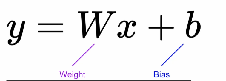
#Weight와 Bias 0으로 초기화(항상 출력0예측)

W = torch.zeros(1, requires_grad = True) #학습할 것 명시
b = torch.zeros(1, requires_grad = True) #학습할 것 명시


hypothesis = x_train * W + b
Compute Loss(Model 학습)
Mean Squared Error(MSE)
정답과 얼마나 가까운지 확인 작업으로 loss계산
실제 Training dataset의 y값 차이를 제곱하여 평균
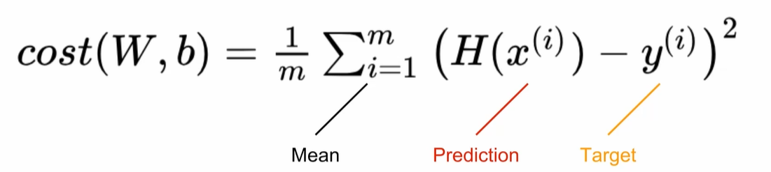
cost = torch.mean((hypothesis - y_train) ** 2)
Gradient descent
-
torch.optim 라이브러리 사용
- [W,b]는 학습할 tensor
- lr = 0.01
-
항상 붙는 3줄(꼭 기억)
- zero_grad()로 gradient초기화
- backward()로 gradient계산
- step()로 계산 #Gradient방향대로 Weight와 Biase, W와 b 계산합니다.
optimizer = torch.optim.SGD([W, b], lr=0.01)

optimizer.zero_grad()
cost.backward()
optimizer.step()
Full training code(Linear regression)
! pip install torchvision

import numpy as np
import torch

#데이터 정의

x_train = torch.FloatTensor([[1], [2], [3]])
y_train = torch.FloatTensor([[2], [4], [6]])


# Hypothesis초기화

W = torch.zeros(1, requires_grad = True)

b = torch.zeros(1, requires_grad = True)


#Optimizer정의

optimizer = torch.optim.SGD([W, b], lr = 0.01)

#Hypothesis 예측

nb_epochs = 1000
for epoch in range(1, nb_epochs + 1):
    hypothesis = x_train * W + b
    cost = torch.mean((hypothesis - y_train) ** 2)

    optimizer.zero_grad()
    cost.backward() #cost계산
    optimizer.step() #Optimizer로 학습
성장을 도울 아카이빙 블로그