[부스트캠프 AI tech DL Basic] week04 (2022.02.08)

03 Optimization

bagging vs boosting

https://medium.com/analytics-vidhya/ensemble-models-bagging-boosting-c33706db0b0b

Gradient Descent Methods

• Stochastic gradient descent
  : update every single sample
• Mini-batch gradient descent
  : update subset of data
• batch gradient descent
  : update whole data

Batchsize

ON LARGE-BATCH TRAINING FOR DEEP LEARNING: GENERALIZATION GAP AND SHARP MINIMA, 2017

"We have observed that the loss function landscape of deep neural
networks is such that large-batch methods are attracted to regions with sharp minimizers and
that, unlike small-batch methods, are unable to escape basins of attraction of these minimizers"

i) LB는 model을 over-fit한다

ii) LB는 saddle point에 attracted된다

iii) LB는 SB에 비해 탐색이 부족하고, initial point에 가까운 minimizer에 zoom-in하는 경향이 있다.

iv) SB와 LB는 다른 minimizer에 수렴한다

*LB: Large-Batch / SB: Small-Batch

*saddle point: 안장점, 어느 방향에서보면 극대값이지만, 다른 방향에서 보면 극소값이 되는 점(wiki)

• batch size별 비교(MNIST)
  
  
• batch size / learning rate 별 비교
  

https://medium.com/mini-distill/effect-of-batch-size-on-training-dynamics-21c14f7a716e

※ It is known that simply increasing the learning rate does not fully compensate for large batch sizes in more complex datasets than MNIST.

Gardient Descent Method

• Nesterov Accelerated Gradient
  
• Adagrad
  
• Adadelta
  
• RMSprop
  
• Adam(Adaptive Moment Estimation)
  
  
  

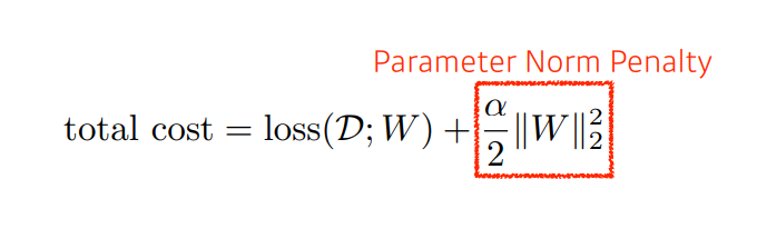
Regularization

• Early Stopping
• Parameter norm penalty(weight decay)
  
  • 파라미터가 너무 커지지 않게함
  • L1(Lasso), L2(Lidge)
  • add smoothness to function space
• Data augmentation
• Noise robustness
• Label smoothing
  
• Dropout
• Batch normalization
  

(03 - 실습) Optimization Methods(colab)

[기본 과제] Optimization Assignment (colab)

04 Convolution은 무엇인가?

• 최근 FC Layer를 줄이는 추세
• 파라미터가 많을 수록 generalization에 불리
• 파라미터 개수에 대한 감을 갖고 있는 것이 중요
  

https://towardsdatascience.com/types-of-convolutions-in-deep-learning-717013397f4d

stride

:window가 건너뛰는 크기

padding

: input의 추가 테두리

convolution Arithmeric

https://seongkyun.github.io/study/2019/01/25/num_of_parameters/

• Dense layer가 Convolution layer에 비해 더 많은 파라미터가 필요하다.
• 앞 단에 convolution layer를 깊게 쌓고, 뒷 단에 FC layer를 줄이는 추세
  
  

1x1 Convolution

• dimension reduction
• increasing depth
• reduce #parameter
• ex) bottlenect architecture

(04 - 실습) Convolutional Neural Network(colab)

05 Modern CNN - 1x1 convolution의 중요성

SOTA models

• AlexNet
  • ReLU
    • linear model의 성질을 보존한다
    • gradient descent를 최적화하기 쉽다
    • vanishing gradient문제를 해결
  • 2 GPU
  • Local response normalization(LRN), Overlapping pooling
  • Data augmentation
  • Dropout
    
    
• VGGNet
  • 3x3 filter만 사용
  • 1x1 convolution for fc layer
  • dropout
  • why 3x3 convolution?
    ※ 3x3을 두번한 것과 5x5를 한번한 것은 동일한 receptive field를 가짐.

*Receptive field: 하나의 feature map 값을 얻기 위해서 고려할 수 있는 input의 크기

• GoogLeNet
  • NIN(network in network) 구조
  • inception block
    
    • 3x3, 5x5 convolution 전에 1x1 conv layer를 거침
    • 파라미터 수를 줄일 수 있음
    • 1x1 convolution은 channel-wise dimension reduction
  • benefit of 1x1 convolution
  1. (h, w, 128) --> (h', w', 128)
  2. (h, w, 128) -> (h, w, 32) -> (h', w', 128)
     * 약 30%의 파라미터 감소
     
     
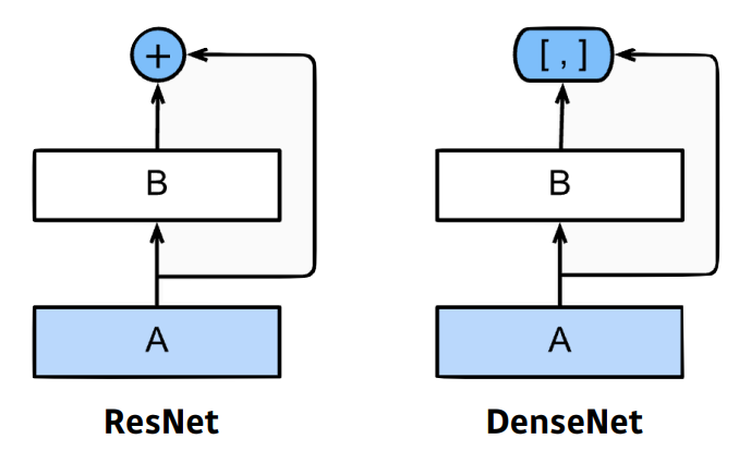
• ResNet
  • identity map(skip connection)
    shorcut의 차원을 맞추기위해 1x1 conv를 사용
    batchnorm의 위치(논문, 사람마다 다름)
    bottleneck architecture
    GooLeNet과 유사
    
    
• DenseNet
  • concatenate
  • Dense Block
    : 모든 feature map을 concatenate
    : channel의 수가 기하급수적으로 증가
  • Transition Block
    : BatchNorm -> 1x1 Conv -> 2x2 AvgPooling
    : Dense Block 다음에 차원을 축소시키는 역할

06 Computer Vision Applications

Semantic Segmentation

- Fully Convolutional Network

• convolutionalization
• dense layer와 파라미터 수는 일치
• 이미지의 크기와 상관없이 사용가능
• heatmap output으로 출력할 수 있음

- Deconvolution

• FCN(Fully Convolutional Network)의 output을 이미지로 upsample하기 위해 사용됨
  
  

Detection

• R-CNN1) takes an input image
  2) extracts around 2,000 region
  proposals (using Selective search)
  3) compute features for each
  proposal(using AlexNet)
  4) classifies with linear SVMs.
  
  
• SPPNet
  • CNN을 한 번 돌려서 R-CNN에 비해 빠름
    
    
• Fast R-CNN
  • ROI pooling
• Faster R-CNN
  • Region Proposal Network(RPN) + Fast R-CNN
  • Fully Convolution Network
    
    
• YOLO
  • bounding box를 뽑는 Region Proposal step이 없어서 빠름
  • 이미지를 SxS grid로 나눔
  • B개의 bbox를 예측
  • bbox의 class와 confidence를 예측