본 자료는 이수안 교수님(https://suanlab.com/)의 자료를 일부 수정 후 업데이트 한 자료입니다.

ipynb 나 pdf 자료가 필요하신분은 연락주세요.

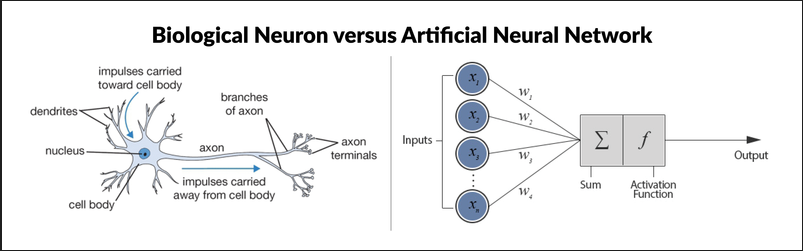
인공신경망(Artificial Neural Network)

• 인간 두뇌에 대한 계산적 모델을 통해 인공지능을 구현하려는 분야
• 인간의 뇌 구조를 모방: 뉴런과 뉴런 사이에는 전기신호를 통해 정보를 전달

생물학적 신경세포와 인공신경망 비교

• 신경세포(Neuron)

  • 수상돌기(樹狀突起, Dendrite) : 다른 신경세포의 축색돌기와 연결되어 전기화학적 신호를 받아들이는 부위
  • 축색돌기(軸索突起, Axon) : 수신한 전기화학적 신호의 합성결과 값이 특정 임계값이 이상이면 신호를 내보는 부위
  • 신경연접(神經連接, Synapse) : 수상돌기와 축색돌기 연결 부위, 전달되는 신호의 증폭 또는 감쇄

• 인공 뉴런(Artificial Neuron)

  • 신경세포 구조를 단순화하여 모델링한 구조
  • 노드(Node)와 엣지(Edge)로 표현
  • 하나의 노드안에서 입력(Inputs)와 가중치(Weights)를 곱하고 더하는 선형구조(linear)
  • 활성화 함수(activation function)를 통한 비선형 구조(non-linear) 표현 가능

• 인공 신경망(Artificial Neural Network)

  • 여러 개의 인공뉴런들이 모여 연결된 형태
  • 뉴런들이 모인 하나의 단위를 층(layer)이라고 하고, 여러 층(multi layer)으로 이루어질 수 있음
  • ex) 입력층(input layer), 은닉층(hidden layer), 출력층(output layer)

  딥러닝 프레임워크(Deep Learning Framework)

  텐서플로우(Tensorflow)

• 가장 널리 쓰이는 딥러닝 프레임워크 중 하나

• 구글이 주도적으로 개발하는 플랫폼

• 파이썬, C++ API를 기본적으로 제공하고,
  자바스크립트(JavaScript), 자바(Java), 고(Go), 스위프트(Swift) 등 다양한 프로그래밍 언어를 지원

• tf.keras를 중심으로 고수준 API 통합 (2.x 버전)

• TPU(Tensor Processing Unit) 지원

  • TPU는 GPU보다 전력을 적게 소모, 경제적
  • 일반적으로 32비트(float32)로 수행되는 곱셈 연산을 16비트(float16)로 낮춤

  케라스(Keras)

• 파이썬으로 작성된 고수준 신경망 API로 TensorFlow, CNTK, 혹은 Theano와 함께 사용 가능
• 사용자 친화성, 모듈성, 확장성을 통해 빠르고 간편한 프로토타이핑 가능
• 컨볼루션 신경망, 순환 신경망, 그리고 둘의 조합까지 모두 지원
• CPU와 GPU에서 매끄럽게 실행

딥러닝 데이터 표현과 연산

• 데이터 표현을 위한 기본 구조로 텐서(tensor)를 사용
• 텐서는 데이터를 담기위한 컨테이너(container)로서 일반적으로 수치형 데이터를 저장

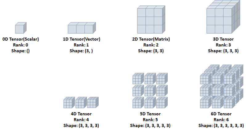
텐서(Tensor)

• Rank: 축의 개수
• Shape: 형상(각 축에 따른 차원 개수)
• Type: 데이터 타입

import tensorflow as tf
import numpy as np

0D Tensor(Scalar)

• 하나의 숫자를 담고 있는 텐서(tensor)
• 축과 형상이 없음

t0 = tf.constant(1) 
print(t0)
print(tf.rank(t0)) # 축이 없는(0) 상태

1D Tensor(Vector)

• 값들을 저장한 리스트와 유사한 텐서
• 하나의 축이 존재

t1 = tf.constant([1,2,3]) 
print(t1)
print(tf.rank(t1))

2D Tensor(Matrix)

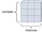
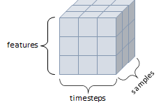
• 행렬과 같은 모양으로 두개의 축이 존재
• 일반적인 수치, 통계 데이터셋이 해당
• 주로 샘플(samples)과 특성(features)을 가진 구조로 사용

t2 = tf.constant([[1,2,3],[4,5,6],[7,8,9]]) 
print(t2)
print(tf.rank(t2))
#tf.Tensor(
#[[1 2 3]
# [4 5 6]
# [7 8 9]], shape=(3, 3), dtype=int32)
#tf.Tensor(2, shape=(), dtype=int32)

3D Tensor

• 큐브(cube)와 같은 모양으로 세개의 축이 존재
• 데이터가 연속된 시퀀스 데이터나 시간 축이 포함된 시계열 데이터에 해당
• 주식 가격 데이터셋, 시간에 따른 질병 발병 데이터 등이 존재
• 주로 샘플(samples), 타임스텝(timesteps), 특성(features)을 가진 구조로 사용

t3 = tf.constant([[[1,2,3],
                   [4,5,6],
                   [7,8,9]],
                  [[1,2,3],
                   [4,5,6],
                   [7,8,9]],
                  [[1,2,3],
                   [4,5,6],
                   [7,8,9]]]) 
print(t3)
print(tf.rank(t3)) # 축이 없는(0) 상태

output :
tf.Tensor(
[[[1 2 3][4 5 6]
[7 8 9]]

[[1 2 3][4 5 6]
[7 8 9]]

[[1 2 3][4 5 6]
[7 8 9]]], shape=(3, 3, 3), dtype=int32)
tf.Tensor(3, shape=(), dtype=int32)

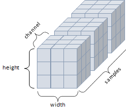
4D Tensor

• 4개의 축
• 컬러 이미지 데이터가 대표적인 사례 (흑백 이미지 데이터는 3D Tensor로 가능)
• 주로 샘플(samples), 높이(height), 너비(width), 컬러 채널(channel)을 가진 구조로 사용

5D Tensor

• 5개의 축
• 비디오 데이터가 대표적인 사례
• 주로 샘플(samples), 프레임(frames), 높이(height), 너비(width), 컬러 채널(channel)을 가진 구조로 사용

텐서 데이터 타입

• 텐서의 기본 dtype
  • 정수형 텐서: int32
  • 실수형 텐서: float32
  • 문자열 텐서: string
• int32, float32, string 타입 외에도 float16, int8 타입 등이 존재
• 연산시 텐서의 타입 일치 필요
• 타입변환에는 tf.cast() 사용

i = tf.constant(2) 
print(i)

output : tf.Tensor(2, shape=(), dtype=int32)

# tf.constant(2.)는 실수형 텐서를 생성
# 기본 dtype은 float32tf.Tensor(2.0, shape=(), dtype=float32)
i = tf.constant(2.) 
print(i)

output : tf.Tensor(2.0, shape=(), dtype=float32)

# tf.constant('ms')는 문자열 텐서를 생성
# 기본 dtype은 string
s = tf.constant('ms')
print(s) # b : 해당 문자열이 바이트(byte) 형식

output : tf.Tensor(b'ms', shape=(), dtype=string)

f16 = tf.constant(2., dtype=tf.float16)
print(f16)

output : tf.Tensor(2.0, shape=(), dtype=float16)

i8 = tf.constant(2, dtype=tf.int8) 
print(i)

output : tf.Tensor(2.0, shape=(), dtype=float32)

f32 = tf.cast(f16, tf.float32)
print(f32)

output : tf.Tensor(2.0, shape=(), dtype=float32)

i32 = tf.cast(i8, tf.int32)
print(i32)

output : tf.Tensor(2, shape=(), dtype=int32)

텐서 연산

# 텐서 연산 예제
# tf.constant()를 사용하여 상수 텐서를 생성하고 기본적인 사칙연산을 수행
# 덧셈과 뺄셈은 + 와 - 연산자 또는 tf.add()와 tf.subtract() 함수를 사용할 수 있음
print(tf.constant(2) + tf.constant(2))
print(tf.constant(2) - tf.constant(2))
print(tf.add(tf.constant(2) , tf.constant(2)))
print(tf.subtract(tf.constant(2) , tf.constant(2)))

output :
tf.Tensor(4, shape=(), dtype=int32)
tf.Tensor(0, shape=(), dtype=int32)
tf.Tensor(4, shape=(), dtype=int32)
tf.Tensor(0, shape=(), dtype=int32)

print(tf.constant(2) * tf.constant(2))
print(tf.constant(2) / tf.constant(2))
print(tf.multiply(tf.constant(2) , tf.constant(2)))
print(tf.divide(tf.constant(2) , tf.constant(2)))

output :
print(tf.constant(2) * tf.constant(2))
print(tf.constant(2) / tf.constant(2))
print(tf.multiply(tf.constant(2) , tf.constant(2)))
print(tf.divide(tf.constant(2) , tf.constant(2)))

# print(tf.constant(2) + tf.constant(2.2)) # 에러남
print(tf.cast(tf.constant(2),tf.float32) + tf.constant(2.2))

output : tf.Tensor(4.2, shape=(), dtype=float32)

딥러닝 구조 및 학습

• 딥러닝 구조와 학습에 필요한 요소
  • 모델(네트워크)를 구성하는 레이어(layer)
  • 입력 데이터와 그에 대한 목적(결과)
  • 학습시에 사용할 피드백을 정의하는 손실 함수(loss function)
  • 학습 진행 방식을 결정하는 옵티마이저(optimizer)

레이어(Layer)

• 신경망의 핵심 데이터 구조
• 하나 이상의 텐서를 입력받아 하나 이상의 텐서를 출력하는 데이터 처리 모듈
• 상태가 없는 레이어도 있지만, 대부분 가중치(weight)라는 레이어 상태를 가짐
• 가중치는 확률적 경사 하강법에 의해 학습되는 하나 이상의 텐서

• Keras에서 사용되는 주요 레이어
  • Dense
  • Activation
  • Flatten
  • Input

https://www.securityinfowatch.com/video-surveillance/video-analytics/article/21069937/deep-learning-to-the-rescue

# tensorflow.keras.layers에서 주요 레이어들을 import
# Dense: 완전연결계층을 구현하는 레이어
# Activation: 활성화 함수를 적용하는 레이어  
# Flatten: 다차원 입력을 1차원으로 펼치는 레이어
# Input: 모델의 입력을 정의하는 레이어
from tensorflow.keras.layers import Dense, Activation, Flatten, Input

Dense

• 완전연결계층(Fully-Connected Layer)

• 노드수(유닛수), 활성화 함수(activation) 등을 지정

• name을 통한 레이어간 구분 가능

• 가중치 초기화(kernel_initializer)

  • 신경망의 성능에 큰 영향을 주는 요소
  • 보통 가중치의 초기값으로 0에 가까운 무작위 값 사용
  • 특정 구조의 신경망을 동일한 학습 데이터로 학습시키더라도, 가중치의 초기값에 따라 학습된 신경망의 성능 차이가 날 수 있음
  • 오차역전파 알고리즘은 기본적으로 경사하강법을 사용하기 때문에 최적해가 아닌 지역해에 빠질 가능성이 있음
  • Keras에서는 기본적으로 Glorot uniform 가중치(Xavier 분포 초기화), zeros bias로 초기화
  • kernel_initializer 인자를 통해 다른 가중치 초기화 지정 가능
  • Keras에서 제공하는 가중치 초기화 종류: https://keras.io/api/layers/initializers/

# 아래 레이어를 통과하면 결과로 10개의 출력 노드가 생성됨.
# Dense 레이어는 이전 레이어의 출력이 어떤 크기든 간에 
# 이를 받아들여 내부적으로 적절히 처리하고 10개의 출력을 생성
# 레이어를 정의할 때 입력 노드의 수를 명시적으로 지정할 필요는 없음.

Dense(10, activation='softmax')
Dense(10, activation='relu', name='Dense Layer')
Dense(10, kernel_initializer='he_normal', name='Dense Layer')

Activation

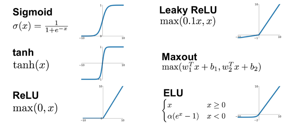
• Dense layer에서 미리 활성화 함수를 지정할 수도 있지만 필요에 따라 별도 레이어를 만들어줄 수 있음
• Keras에서 제공하는 활성화 함수(activation function) 종류: https://keras.io/ko/activations/

# 사용 예시
dense = Dense(10,activation='relu',name='Dense Layer')
Activation(dense)

Flatten

• 배치 크기(또는 데이터 크기)를 제외하고 데이터를 1차원으로 쭉 펼치는 작업
• 예시)
  (128, 3, 2, 2) -> (128, 12)
  

# 전체 출력은 (batch_size, height * width * channels) 형태를 가짐. 
# 여기서 첫 번째 차원은 배치 크기를 나타내고, 두 번째 차원은 평탄화된 피처를 나타냄.
# 따라서, Flatten 레이어의 출력 텐서는 랭크가 2인 2D 텐서임.
flatten = Flatten(input_shape=(128,3,2,2))

### Input

- 모델의 입력을 정의
- `shape`, `dtype`을 포함
- 하나의 모델은 여러 개의 입력을 가질 수 있음
- `summary()` 메소드를 통해서는 보이지 않음

# None: 이 위치의 None은 배치 크기(batch size)를 나타냅니다.
# None이 사용된 이유는 배치 크기가 미리 정의되지 않았고,
# 모델을 실행할 때 어떤 배치 크기도 사용될 수 있음을 의미함.
# 즉, 입력 데이터의 총 수는 가변적이며, 실제 모델 훈련이나 추론시에 결정됩니다.

Input(shape=(8,), dtype=tf.int32)

모델(Model)

• 딥러닝 모델은 레이어로 만들어진 비순환 유향(방향이 있는) 그래프(Directed Acyclic Graph, DAG) 구조

모델 구성

• Sequential()
• 서브클래싱(Subclassing) - 클래스를 상속받아서 하는 방법
• 함수형 API

Sequential()

• 모델이 순차적인 구조로 진행할 때 사용
• 간단한 방법
  • Sequential 객체 생성 후,add()를 이용한 방법
  • Sequential 인자에 한번에 추가 방법
• 다중 입력 및 출력이 존재하는 등의 복잡한 모델을 구성할 수 없음

from tensorflow.keras.layers import Dense, Input, Flatten
from tensorflow.keras.models import Sequential, Model
from tensorflow.keras.utils import plot_model

model = Sequential()
model.add(Input(shape=(28,28)))
model.add(Dense(300, activation='relu'))
model.add(Dense(100, activation='relu'))
model.add(Dense(10, activation='softmax'))
model.summary()

output :

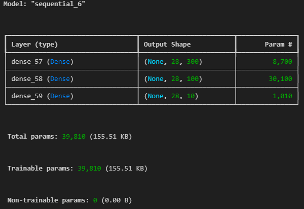
Param = 가중치(weight, biases)의 총 수
가중치의 총 수 = (입력 유닛 수) x (출력 유닛 수)
바이어스의 총 수 = 출력 유닛 수(각 출력 유닛마다 하나의 바이어스가 있음)
총 파라미터 수 = 가중치의 총 수 + 바이어스의 총 수

dense_4 = 28300+300
dense_5 = 300100+100
dense_6 = 100*10+10

#!pip install pydot
plot_model(model)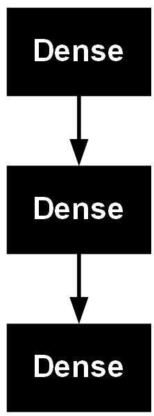

model = Sequential([
    Input(shape=(28,28)),
    Dense(300, activation='relu'),
    Dense(100, activation='relu'),
    Dense(10, activation='softmax')])
model.summary()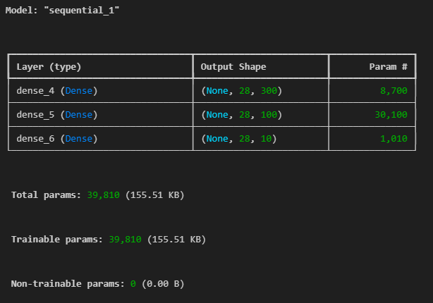

함수형 API

• 가장 권장되는 방법(sequential은 단순하게 순차적으로 쌓이는 구조에서만 동작 가능)
• 모델을 복잡하고, 유연하게 구성 가능
• 다중 입출력을 다룰 수 있음

inputs = Input(shape=(28,28,1))
x = Flatten(input_shape=(28,28,1))(inputs)
x = Dense(300,activation='relu')(x)
x = Dense(100,activation='relu')(x)
x = Dense(10,activation='softmax')(x)

model = Model(inputs=inputs, outputs=x)
model.summary()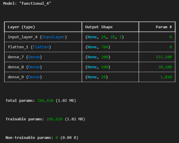

plot_model(model)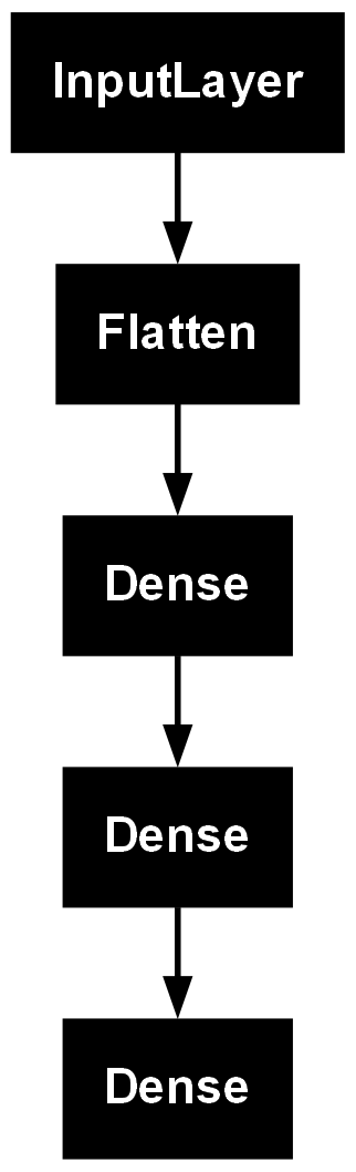

# 복잡한 모델
from tensorflow.keras.layers import Concatenate

input_layer = Input(shape=(28,28))
hidden1 = Dense(100, activation='relu')(input_layer)
hidden2 = Dense(30, activation='relu')(hidden1)
concat = Concatenate()([input_layer, hidden2])
output = Dense(1)(concat)

model = Model(inputs=[input_layer], outputs=[output])
model.summary()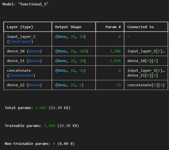

plot_model(model)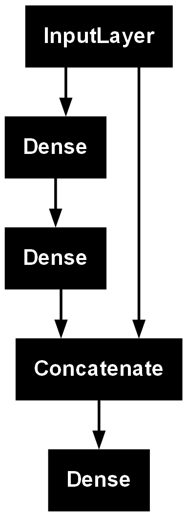

# input 두개인 모델
input_1 = Input(shape=(10,10))
input_2 = Input(shape=(10,28))

hidden1 = Dense(100, activation='relu')(input_2)
hidden2 = Dense(10, activation='relu')(hidden1)
concat = Concatenate()([input_1, hidden2])

output = Dense(1, activation='sigmoid')(concat)
model = Model(inputs=[input_1, input_2], outputs=[output])
model.summary()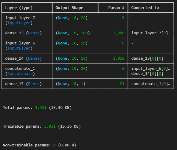

plot_model(model)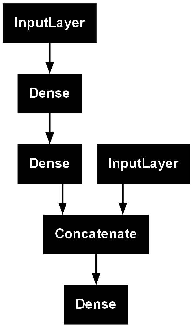

# input 두개인 모델
input_ = Input(shape=(10,10), name = 'input_')

hidden1 = Dense(100, activation='relu')(input_)
hidden2 = Dense(10, activation='relu')(hidden1)

output = Dense(1, activation='sigmoid', name='main_output')(hidden2)
sub_output = Dense(1, name='sub_output')(hidden2)

model = Model(inputs=[input_], outputs=[output, sub_output])
model.summary()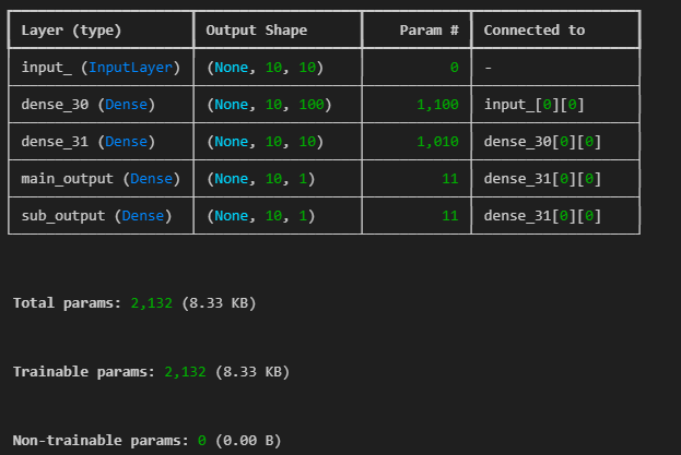

plot_model(model)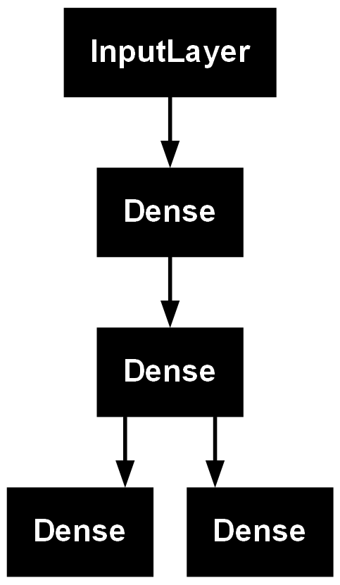

# input, output 둘 다 두개인 모델
input_1 = Input(shape=(10,10))
input_2 = Input(shape=(10,28))

hidden1 = Dense(100, activation='relu')(input_2)
hidden2 = Dense(10, activation='relu')(hidden1)
concat = Concatenate()([input_1, hidden2])

output = Dense(1, activation='sigmoid',name='main_output')(concat)
sub_out = Dense(1,name='sub_output')(hidden2)

model = Model(inputs=[input_1, input_2], outputs=[output, sub_out])
model.summary()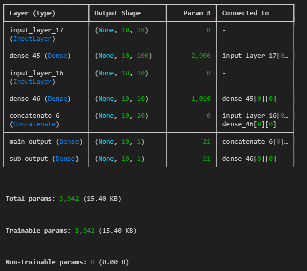

plot_model(model ,show_layer_names=True, show_shapes=True)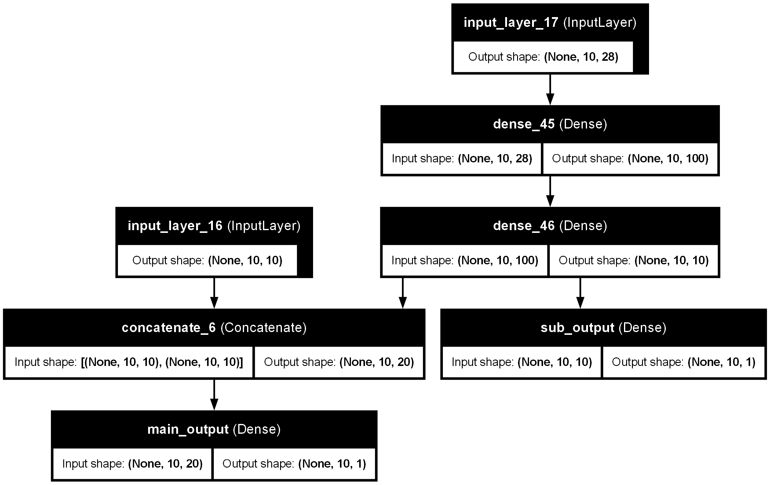

#### 서브클래싱(Subclassing)

- 커스터마이징에 최적화된 방법
- 이미 어느정도 만들어진걸 조금 수정하여 재활용하는 느낌
- Model 클래스를 상속받아 Model이 포함하는 기능을 사용할 수 있음  
  - `fit()`, `evaluate()`, `predict()`
  - `save()`, `load()`
- 주로 `call()` 메소드안에서 원하는 계산 가능
  - for, if, 저수준 연산 등
- 권장되는 방법은 아니지만 어떤 모델의 구현 코드를 참고할 때, 해석할 수 있어야함

모델 가중치 확인

class MyModel(Model):
    def __init__(self, units=30, activation='relu',**kwargs):
        # Model class의 생성자 실행. Model class에 정의된 value 속성도 초기화
        super(MyModel, self).__init__(**kwargs)
        #super().__init__(**kwargs) # 이렇게 가능
        self.dense_layer1 = Dense(300, activation=activation)
        self.dense_layer2 = Dense(100, activation=activation)
        self.dense_layer3 = Dense(units, activation=activation)
        self.output_layer = Dense(10, activation='softmax')
   
    def call(self, inputs):
        x = self.dense_layer1(x)
        x = self.dense_layer2(x)
        x = self.dense_layer3(x)
        x = self.output_layer(x)
        return x
    
model = MyModel()
# 참고
# def abc(**kwargs):
#     print(kwargs)
# abc(a=3, b='c') # {'a': 3, 'b': 'c'}

inputs = Input(shape=(28,28,1))
x = Flatten(input_shape=(28,28,1))(inputs)
x = Dense(300, activation='relu')(x)
x = Dense(100, activation='relu')(x)
x = Dense(10, activation='softmax')(x)

model = Model(inputs=inputs, outputs = x)
model.summary()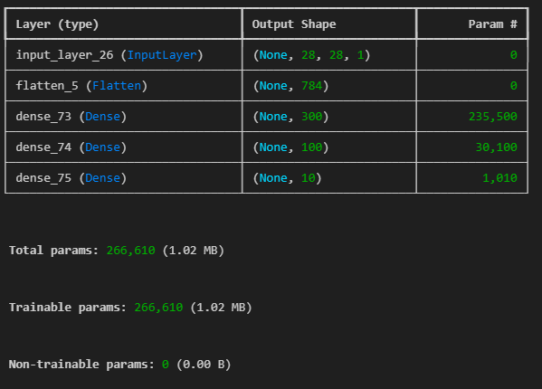

model.layers

output:
[<InputLayer name=input_layer_26, built=True>,
 <Flatten name=flatten_5, built=True>,
 <Dense name=dense_73, built=True>,
 <Dense name=dense_74, built=True>,
 <Dense name=dense_75, built=True>]

hidden_2 = model.layers[2]
hidden_2.name

output : 'dense_73'

# 가져온 모델 맞는지 검증하기
model.get_layer('dense_73') == hidden_2

output : True

# 레이어의 weight, bias 확인하기
weights, biases = hidden_2.get_weights()
print(weights.shape)
print(biases.shape)

output :
(784, 300)
(300,)

print(weights)

output:
[[-0.0189958 0.04178642 -0.02973261 ... 0.02392814 -0.06515371
-0.01094473][-0.06765752 0.05939554 0.05841401 ... -0.03066007 0.07289664 0.03665416]
[ 0.02429469 0.06326848 0.03675973 ... -0.06022335 0.03570367
0.04572336]
...
[ 0.03738911 0.0086766 -0.05104835 ... 0.03970996 -0.00280691
-0.06960735][ 0.06139068 0.00252346 -0.00775075 ... 0.05078986 -0.03957617 0.0160888 ]
[ 0.06548205 0.01272491 -0.05994889 ... -0.05388444 0.06571051
-0.02650245]]

print(biases)

output:
[0. 0. 0. 0. 0. 0. 0. 0. 0. 0. 0. 0. 0. 0. 0. 0. 0. 0. 0. 0. 0. 0. 0. 0.
0. 0. 0. 0. 0. 0. 0. 0. 0. 0. 0. 0. 0. 0. 0. 0. 0. 0. 0. 0. 0. 0. 0. 0.
0. 0. 0. 0. 0. 0. 0. 0. 0. 0. 0. 0. 0. 0. 0. 0. 0. 0. 0. 0. 0. 0. 0. 0.
0. 0. 0. 0. 0. 0. 0. 0. 0. 0. 0. 0. 0. 0. 0. 0. 0. 0. 0. 0. 0. 0. 0. 0.
0. 0. 0. 0. 0. 0. 0. 0. 0. 0. 0. 0. 0. 0. 0. 0. 0. 0. 0. 0. 0. 0. 0. 0.
0. 0. 0. 0. 0. 0. 0. 0. 0. 0. 0. 0. 0. 0. 0. 0. 0. 0. 0. 0. 0. 0. 0. 0.
0. 0. 0. 0. 0. 0. 0. 0. 0. 0. 0. 0. 0. 0. 0. 0. 0. 0. 0. 0. 0. 0. 0. 0.
0. 0. 0. 0. 0. 0. 0. 0. 0. 0. 0. 0. 0. 0. 0. 0. 0. 0. 0. 0. 0. 0. 0. 0.
0. 0. 0. 0. 0. 0. 0. 0. 0. 0. 0. 0. 0. 0. 0. 0. 0. 0. 0. 0. 0. 0. 0. 0.
0. 0. 0. 0. 0. 0. 0. 0. 0. 0. 0. 0. 0. 0. 0. 0. 0. 0. 0. 0. 0. 0. 0. 0.
0. 0. 0. 0. 0. 0. 0. 0. 0. 0. 0. 0. 0. 0. 0. 0. 0. 0. 0. 0. 0. 0. 0. 0.
0. 0. 0. 0. 0. 0. 0. 0. 0. 0. 0. 0. 0. 0. 0. 0. 0. 0. 0. 0. 0. 0. 0. 0.
0. 0. 0. 0. 0. 0. 0. 0. 0. 0. 0. 0.]

### 모델 컴파일(compile)
#- 모델을 구성한 후, 사용할 손실 함수(loss function), 옵티마이저(optimizer)를 지정
model.compile(loss = 'sparse_categorical_crossentropy',
              optimizer='sgd',
              metrics = ['accuracy'])

손실 함수(Loss Function)

• 학습이 진행되면서 해당 과정이 얼마나 잘 되고 있는지 나타내는 지표
• 모델이 훈련되는 동안 최소화될 값으로 주어진 문제에 대한 성공 지표
• 손실 함수에 따른 결과를 통해 학습 파라미터를 조정
• 최적화 이론에서 최소화 하고자 하는 함수
• 미분 가능한 함수 사용
• Keras에서 주요 손실 함수 제공
  • sparse_categorical_crossentropy: 클래스가 배타적 방식으로 구분, 즉 (0, 1, 2, ..., 9)와 같은 방식으로 구분되어 있을 때 사용
  • categorical_cross_entropy: 클래스가 원-핫 인코딩 방식으로 되어 있을 때 사용
  • binary_crossentropy: 이진 분류를 수행할 때 사용

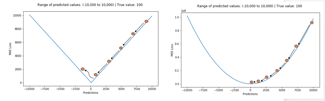
평균절대오차(Mean Absolute Error, MAE)

• 오차가 커져도 손실함수가 일정하게 증가
• 이상치(Outlier)에 강건함(Robust)
  • 데이터에서 [입력 - 정답] 관계가 적절하지 않은 것이 있을 경우에, 좋은 추정을 하더라도 오차가 발생하는 경우가 발생
  • 해당 이상치에 해당하는 지점에서 손실 함수의 최소값으로 가는 정도의 영향력이 크지 않음
• 회귀 (Regression)에 많이 사용
• 평균절대오차 식:
  $ \qquad \qquad E = \frac{1}{n}\sum_{i=1}^n \left | y_i - \tilde{y}_i \right |$
  • $y_i$ : 학습 데이터의 $i\ $번째 정답
  • $\tilde{y}_i$ : 학습 데이터의 입력으로 추정한 $i\ $번째 출력

평균제곱오차(Mean Squared Error, MSE)

• 가장 많이 쓰이는 손실 함수 중 하나
• 오차가 커질수록 손실함수가 빠르게 증가
  • 정답과 예측한 값의 차이가 클수록 더 많은 페널티를 부여
• 회귀 (Regression)에 쓰임
• 평균제곱오차 식: $ \qquad \qquad E = \frac{1}{n}\sum_{i=1}^n ( y_i - \tilde{y}_i)^2 $
  • $y_i$ : 학습 데이터의 $i\ $번째 정답
  • $\tilde{y}_i$ : 학습 데이터의 입력으로 추정한 $i\ $번째 출력

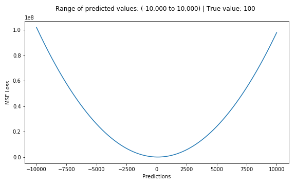
손실함수 MAE와 MSE 비교

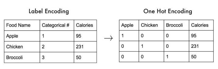
원-핫 인코딩(One-Hot Encoding)

• 범주형 변수를 표현할 때 사용
• 가변수(Dummy Variable)이라고도 함
• 정답인 레이블을 제외하고 0으로 처리

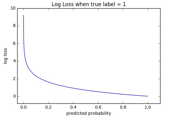
교차 엔트로피 오차(Cross Entropy Error, CEE)

• 이진 분류(Binary Classification), 다중 클래스 분류(Multi Class Classification)
• 소프트맥스(softmax)와 원-핫 인코딩(ont-hot encoding) 사이의 출력 간 거리를 비교
• 정답인 클래스에 대해서만 오차를 계산
• 정답을 맞추면 오차가 0, 틀리면 그 차이가 클수록 오차가 무한히 커짐
• $y = log(x)$
  • $x$가 1에 가까울수록 0에 가까워짐
  • $x$가 0에 가까울수록 $y$값은 무한히 커짐

• 교차 엔트로피 오차 식: $ \qquad \qquad E = - \frac{1}{N}\sum{n} \sum{i} y_i\ log\tilde{y}_i $

  • $y_i$ : 학습 데이터의 $i\ $번째 정답 (원-핫 인코딩, one-hot encoding)
  • $\tilde{y}_i$ : 학습 데이터의 입력으로 추정한 $i\ $번째 출력
  • $N$ : 전체 데이터의 개수
  • $i$ : 데이터 하나당 클래스 개수

• 정답 레이블($y_i$)은 원-핫 인코딩으로 정답인 인덱스에만 1이고, 나머지는 모두 0이라서 다음과 같이 나타낼 수 있음

  $ \qquad \qquad E = - log\tilde{y}_i $

  • 소프트맥스를 통해 나온 신경망 출력이 0.6이라면 $\ -log0.6 \fallingdotseq -0.51\ $이 되고, 신경망 출력이 0.3이라면 $\ -log0.3 \fallingdotseq -1.2\ $이 됨
  • 정답에 가까워질수록 오차값은 작아짐
  • 학습시, 원-핫 인코딩에 의해 정답 인덱스만 살아 남아 비교하지만, 정답이 아닌 인덱스들도 학습에 영향을 미침. 왜냐하면 다중 클래스 분류는 소프트맥스(softmax) 함수를 통해 전체 항들을 모두 다루기 때문

이진 분류 문제의 교차 크로스 엔트로피(Binary Cross Entropy, BCE)

• 이진 분류 문제(Binary Classification Problem)에서도 크로스 엔트로피 오차를 손실함수로 사용 가능
  $ \qquad \qquad E = - \sum_{i=1}^2 y_i\ log\tilde{y}_i \
  \qquad \qquad \ \ \ = -y_1\ log\ \tilde{y}_1 - (1 - y_1)log(1-\ \tilde{y}_1) $
  $\qquad \qquad \qquad ( \because y_2 = 1 - y_1)$
  • $y_i$ : 학습 데이터의 $i\ $번째 정답 (원-핫 인코딩, one-hot encoding)
  • $\tilde{y}_i$ : 학습 데이터의 입력으로 추정한 $i\ $번째 출력

옵티마이저(Optimizer)

• 손실 함수를 기반으로 모델이 어떻게 업데이트되어야 하는지 결정 (특정 종류의 확률적 경사 하강법 구현)
• Keras에서 여러 옵티마이저 제공
  • keras.optimizer.SGD(): 기본적인 확률적 경사 하강법
  • keras.optimizer.Adam(): 자주 사용되는 옵티마이저
  • Keras에서 사용되는 옵티마이저 종류: https://keras.io/ko/optimizers/
• 보통 옵티마이저의 튜닝을 위해 따로 객체를 생성하여 컴파일

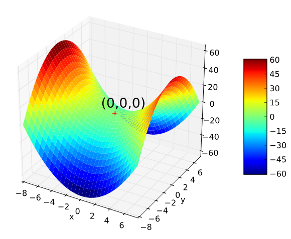
볼록함수(Convex Function)와 비볼록함수(Non-Convex Function)

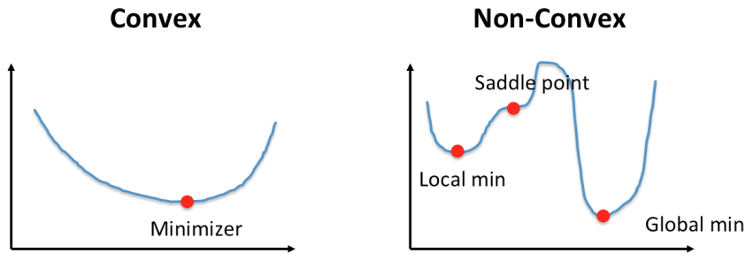
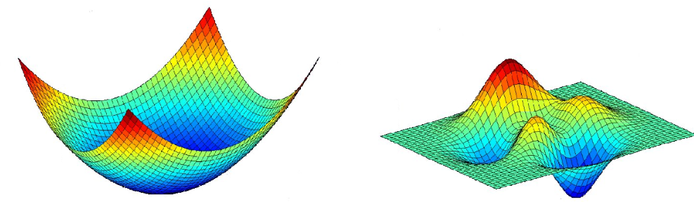
• 볼록함수(Convex Function)
  • 어떤 지점에서 시작하더라도 최적값(손실함수가 최소로하는 점)에 도달할 수 있음
• 비볼록함수(Non-Convex Function)
  • 비볼록 함수는 시작점 위치에 따라 다른 최적값에 도달할 수 있음

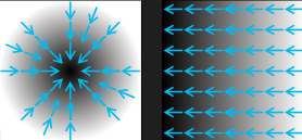
경사하강법(Gradient Decent)

• 미분과 기울기
  • 스칼라를 벡터로 미분한 것(스칼라 함수의 각 변수에 대한 변미분값들을 모아둔 리스트, 즉 그라디언트 벡터를 의미)
  • 그라디언트 벡터 ∇f(x)=[ f'(x1), f'(x2), f'(x3)]
  • w new =w−η⋅∇L(w) 예시) 기존 가중치 벡터[0,0,0,0,0], 그라디언트벡터[1,2,3,4,5], 업데이트후 [-1,-2,-3,-4,-5]

$\quad \frac{df(x)}{dx} = \lim_{\triangle x \to 0} \frac{f(x+\triangle x) - f(x)}{\triangle x}$

$\quad \triangledown f(x) = \left( \frac{\partial f}{\partial x_1}, \frac{\partial f}{\partial x_2},\ ... \ , \frac{\partial f}{\partial x_N} \right)$

• 변화가 있는 지점에서는 미분값이 존재하고, 변화가 없는 지점은 미분값이 0
• 미분값이 클수록 변화량이 크다는 의미

• 경사하강법의 과정

• 경사하강법은 한 스텝마다의 미분값에 따라 이동하는 방향을 결정

• $f(x)$의 값이 변하지 않을 때까지 반복

  $\qquad x_n = x_{n-1} - \eta \frac{\partial f}{\partial x}$

  • $\eta$ : 학습률(learning rate)

• 즉, 미분값이 0인 지점을 찾는 방법

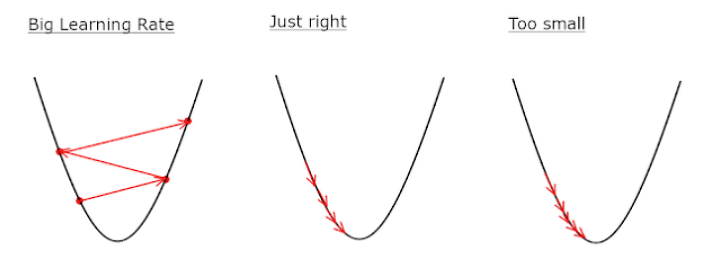
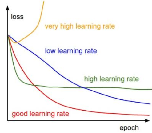
학습률(learning rate)

• 적절한 학습률을 지정해야 최저점에 잘 도달할 수 있음
• 학습률이 너무 크면 발산하고, 너무 작으면 학습이 오래 걸리거나 최저점에 도달하지 않음

안장점(Saddle Point)

• 기울기가 0이지만 극값이 되지 않음
• 경사하강법은 안장점에서 벗어나지 못함

지표(Metrics)

• 모니터링할 지표
• mae나 accuracy 사용
• 줄여서 acc로도 사용 가능
• Keras에서 사용되는 지표 종류: https://keras.io/ko/metrics/

모델 학습, 평가 및 예측

• fit()

  • x: 학습 데이터
  • y: 학습 데이터 정답 레이블
  • epochs: 학습 회수
  • batch_size: 단일 배치에 있는 학습 데이터의 크기
  • validation_data: 검증을 위한 데이터

• evaluate()

  • 테스트 데이터를 이용한 평가

• predict()

  • 임의의 데이터를 사용해 예측

  오차역전파 (Backpropagation)

• 오차역전파 알고리즘

  • 학습 데이터로 정방향(forward) 연산을 통해 손실함수 값(loss)을 구함
  • 각 layer별로 역전파학습을 위해 중간값을 저장
  • 손실함수를 학습 파라미터(가중치, 편향)로 미분하여 마지막 layer로부터 앞으로 하나씩 연쇄법칙을 이용하여 미분
  • 각 layer를 통과할 때마다 저장된 값을 이용
  • 오류(error)를 전달하면서 학습 파라미터를 조금씩 갱신

• 오차역전파 학습의 특징

  • 손실함수를 통한 평가를 한 번만 하고, 연쇄법칙을 이용한 미분을 활용하기 때문에 학습 소요시간이 매우 단축
  • 미분을 위한 중간값을 모두 저장하기 때문에 메모리를 많이 사용

• 신경망 학습에 있어서 미분가능의 중요성

  • 경사하강법(Gradient Descent)에서 손실 함수(cost function)의 최소값, 즉, 최적값을 찾기 위한 방법으로 미분을 활용
  • 미분을 통해 손실 함수의 학습 매개변수(trainable parameter)를 갱신하여 모델의 가중치의 최적값을 찾는 과정

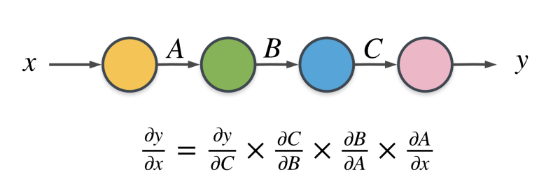
• 합성함수의 미분 (연쇄법칙, chain rule)

  $\qquad \frac{d}{dx} [f(g(x))] = f^\prime(g(x))g^\prime(x)$

  • 여러개를 연속으로 사용 가능

    $ \quad \frac{\partial f}{\partial x} = \frac{\partial f}{\partial u} \times \frac{\partial u}{\partial m} \times \frac{\partial m}{\partial n} \times \ ... \ \frac{\partial l}{\partial k} \times \frac{\partial k}{\partial g} \times \frac{\partial g}{\partial x}
    $

  • 각각에 대해 *편미분 적용가능

  • 편미분 : 다변수 함수에서 하나의 변수를 제외한 나머지 변수들을 상수로 취급하고, 해당 변수에 대해서만 미분을 수행하는 것
    

• 오차역전파의 직관적 이해

  • 학습을 진행하면서, 즉 손실함수의 최소값(minimum)을 찾아가는 과정에서 가중치 또는 편향의 변화에 따라 얼마나 영향을 받는지 알 수 있음