3장 그래프와 워드 클라우드

들어가기에 앞서

해당 글은 "파이썬 텍스트 마이닝 완벽 가이드"를 기반으로 작성되었습니다.

일반인들이 텍스트 분석이라는 이름으로 흔하게 접하게 되는 것은 복잡한 머신러닝이나 딥러닝 모형보다는 빈도를 바탕으로 한 그래프와 워드 클라우드인 경우가 많습니다. 텍스트 분석에서 기본적인 아이디어는 가장 많이 사용된 단어를 파악하는 것입니다.

많은 문서를 탐독하며 공통된 주제나 많이 나온 키워드를 찾는 것은 어렵습니다. 이럴 때 유용하게 쓸 수 있는 가장 기초적인 도구가 단어 빈도를 그래프로 표현하거나 워드 클라우드를 그리는 것입니다.

3.1 단어 빈도 그래프 - 많이 쓰인 단어는?

단어 빈도 그래프를 그리려면, 단어의 빈도를 구해야 합니다. 그러나 그보다 먼저 문서들로부터 각 단어들을 분리해내야 합니다.

실습할 문서는 구텐베르크 프로젝트에서 가져온 이상한 나라의 엘리스 입니다. NLTK에서는 패키지 안에서 구텐베르크 프로젝트의 일부 책들을 제공하고 있습니다. 한 번 어떤 책들이 있는지 확인해봅시다.

import nltk
nltk.download('gutenberg')

from nltk.corpus import gutenberg
file_names = gutenberg.fileids()

print(file_names)

실행 결과

['austen-emma.txt', 'austen-persuasion.txt', 'austen-sense.txt', 'bible-kjv.txt', 'blake-poems.txt', 'bryant-stories.txt', 'burgess-busterbrown.txt', 'carroll-alice.txt', 'chesterton-ball.txt', 'chesterton-brown.txt', 'chesterton-thursday.txt', 'edgeworth-parents.txt', 'melville-moby_dick.txt', 'milton-paradise.txt', 'shakespeare-caesar.txt', 'shakespeare-hamlet.txt', 'shakespeare-macbeth.txt', 'whitman-leaves.txt']

gutenberg.open()으로 파일 제목을 넣어 해당 파일을 열 수 있으며, read()로 내용을 읽을 수 있습니다.

doc_alice = gutenberg.open('carroll-alice.txt').read()
print("Text len:", len(doc_alice))
print("Text sample: ")
print(doc_alice[:500])

실습 결과

Text len: 144395
Text sample: 
[Alice's Adventures in Wonderland by Lewis Carroll 1865]

CHAPTER I. Down the Rabbit-Hole

Alice was beginning to get very tired of sitting by her sister on the
bank, and of having nothing to do: once or twice she had peeped into the
book her sister was reading, but it had no pictures or conversations in
it, 'and what is the use of a book,' thought Alice 'without pictures or
conversation?'

So she was considering in her own mind (as well as she could, for the
hot day made her feel very sleepy an

NLTK를 활용하여 토큰화 해봅시다.

from nltk import word_tokenize
tokens = word_tokenize(doc_alice)

print("Nbr of tokens:", len(tokens))
print("Tokens sample:")
print(tokens[:20])

실행 결과

Nbr of tokens: 33494
Tokens sample:
['[', 'Alice', "'s", 'Adventures', 'in', 'Wonderland', 'by', 'Lewis', 'Carroll', '1865', ']', 'CHAPTER', 'I', '.', 'Down', 'the', 'Rabbit-Hole', 'Alice', 'was', 'beginning']

이제 스테밍을 진행합니다. 여기서는 포터 스테머를 사용합니다.

from nltk.stem import PorterStemmer
stemmer = PorterStemmer()

stem_tokens_alice = [stemmer.stem(token) for token in tokens_alice]

print("Nbr of tokens after stemming:", len(stem_tokens_alice))
print("Tokens sample:")
print(stem_tokens_alice[:20])

실행 결과

Nbr of tokens after stemming: 33494
Tokens sample:
['[', 'alic', "'s", 'adventur', 'in', 'wonderland', 'by', 'lewi', 'carrol', '1865', ']', 'chapter', 'i', '.', 'down', 'the', 'rabbit-hol', 'alic', 'wa', 'begin']

이제 WordNetLemmatizer를 사용하여 표제어를 추출합시다.

from nltk.stem import WordNetLemmatizer
lemmatizer = WordNetLemmatizer()

lem_tokens_alice = [lemmatizer.lemmatize(token) for token in tokens_alice]

print("Nbr of tokens after lammatization:", len(lem_tokens_alice))
print("Tokens sample:")
print(lem_tokens_alice[:20])

실행 결과

Nbr of tokens after lammatization: 33494
Tokens sample:
['[', 'Alice', "'s", 'Adventures', 'in', 'Wonderland', 'by', 'Lewis', 'Carroll', '1865', ']', 'CHAPTER', 'I', '.', 'Down', 'the', 'Rabbit-Hole', 'Alice', 'wa', 'beginning']

위 결과를 종합적으로 볼 때 어간 추출이든, 표제어 추출이든 토큰 수는 변하지 않습니다. 당연하게도 토큰화한 결과에 대해 개별적으로 어간 추출과 표제어 추출을 진행했기 때문입니다. 정규표현식을 이용하여 토큰화를 하고 결과를 비교해봅시다.

from nltk.tokenize import RegexpTokenizer
tokenizer = RegexpTokenizer(r"[\w']{3,}")

reg_tokens_alice = tokenizer.tokenize(doc_alice.lower())
print("Nbr of tokens with RegexpTokenizer:", len(reg_tokens_alice))
print("Tokens sample:")
print(reg_tokens_alice[:20])

실행 결과

Nbr of tokens with RegexpTokenizer: 21616
Tokens sample:
["alice's", 'adventures', 'wonderland', 'lewis', 'carroll', '1865', 'chapter', 'down', 'the', 'rabbit', 'hole', 'alice', 'was', 'beginning', 'get', 'very', 'tired', 'sitting', 'her', 'sister']

기존보다 토큰 수가 현저히 줄어든 것을 알 수 있습니다. ,와 같은 부호가 사라졌을 뿐 아니라 2자 이하의 글자들이 모두 제외되었기 때문입니다.
여기에서는 RegexpTokenizer를 활용한 결과를 사용하는 것으로 하고 불용어를 제거합니다.

from nltk.corpus import stopwords
eng_stops = set(stopwords.words('english'))

result_alice = [word for word in reg_tokens_alice if word not in eng_stops]

print("Nbr of tokens after stopword slemination:", len(result_alice))
print("Tokens sample:")
print(result_alice[:20])

실행 결과

Nbr of tokens after stopword slemination: 12999
Tokens sample:
["alice's", 'adventures', 'wonderland', 'lewis', 'carroll', '1865', 'chapter', 'rabbit', 'hole', 'alice', 'beginning', 'get', 'tired', 'sitting', 'sister', 'bank', 'nothing', 'twice', 'peeped', 'book']

텍스트 전처리가 완료되었으므로 각 단어별로 빈도를 계산해봅시다. 여기서는 딕셔너리로 단어별 개수를 세고, 빈도가 큰 순으로 정렬합니다.

alice_word_count = dict()
for word in result_alice:
    alice_word_count[word] = alice_word_count.get(word, 0) + 1

print("Nbr of use words:", len(alice_word_count))

sorted_word_count = sorted(alice_word_count, key=alice_word_count.get, reverse=True)

print("Top 20 high frequency words:")
for key in sorted_word_count[:20]:
    print(f"{repr(key)}: {alice_word_count[key]}", end=',')

실행 결과

Nbr of use words: 2687
Top 20 high frequency words:
'said': 462,'alice': 385,'little': 128,'one': 98,'know': 88,'like': 85,'went': 83,'would': 78,'could': 77,'thought': 74,'time': 71,'queen': 68,'see': 67,'king': 61,'began': 58,'turtle': 57,"'and": 56,'way': 56,'mock': 56,'quite': 55,

결과를 보면, 'would', 'could'등의 단어는 필요하지 않은 것으로 느껴집니다. 따라서 품사태깅을 이용하여 명사, 동사, 형용사만을 추출해봅니다.

my_tag_list = ['NN', 'VB', 'VBD', 'JJ']
my_words = [word for word, tag in nltk.pos_tag(result_alice) if tag in my_tag_list]

alice_word_count = dict()
for word in my_words:
    alice_word_count[word] = alice_word_count.get(word, 0) + 1

print("Nbr of use words:", len(alice_word_count))

sorted_word_count = sorted(alice_word_count, key=alice_word_count.get, reverse=True)

print("Top 20 high frequency words:")
for key in sorted_word_count[:20]:
    print(f"{repr(key)}: {alice_word_count[key]}", end=',')

실행 결과

Nbr of use words: 2687
Top 20 high frequency words:
'said': 462,'alice': 385,'little': 128,'one': 98,'know': 88,'like': 85,'went': 83,'would': 78,'could': 77,'thought': 74,'time': 71,'queen': 68,'see': 67,'king': 61,'began': 58,'turtle': 57,"'and": 56,'way': 56,'mock': 56,'quite': 55,

이제 그래프를 이용하여 시각화 해봅시다. 여기서 사용할 라이브러리는 matplotlib입니다.

import matplotlib.pyplot as plt
%matplotlib inline

w = [alice_word_count[key] for key in sorted_word_count]

plt.plot(w)
plt.show()

실행 결과

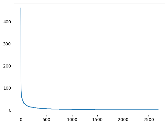
위의 그래프에는 많은 문제점이 있습니다. 이는 다음과 같습니다.

1. 무슨 단어인지 보이지 않습니다.
2. 그래프에 표시된 단어가 너무 많아 단어를 출력한다 하여도 가독성이 전혀 없을 것으로 예상됩니다.

따라서 상위 빈도수 단어들에 대해서만 그려야 합니다.

지프의 법칙
그러나 이 그래프는 많은 통찰을 줍니다. 상위 몇 개의 단어는 빈도수가 매우 높지만 순위가 100위만 넘어가도 매우 적은 빈도수를 보이고 있습니다.
바로 지프의 법칙입니다. 지프는 말무치의 단어들을 사용 빈도가 높은 순서대로 나열하면 단어의 사용 빈도는 단어의 순위에 반비례함을 알아냈습니다. 또한 이는 언어와 관련 없는 도시의 인구 순위, 소득 순위 같은 분야에도 적용됩니다.

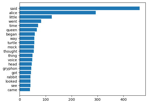
다시 돌아와서 , 우리는 빈도가 높은 상위 단어들을 봄으로써 텍스트의 내용에 대한 통찰을 얻으려고 하는 것이므로 다음과 같이 코드를 수정합니다. 일반적인 막대 그래프를 그리면 단어가 그래프 하단에 표시되고, 이렇게 되면 필연적으로 단어들이 겹치게 됩니다. 따라서 수평 그래프를 이용합니다. 또한 앞에 있는 단어가 원점에 가까운 아래부터 출력되므로, 역순으로 정렬 후 그려줍니다.

책에 있는 그대로 작성하니 오류가 있어 다음을 참조하여 코드를 고쳤습니다.

n = sorted_word_count[:20][::-1]
w = [alice_word_count[key] for key in n]

plt.barh(n, w)
plt.show()

실행 결과

3.2 워드 클라우드로 내용 한눈에 보기

워드 클라우드는 텍스트 분석 결과를 보여주는 시각화 도구 중 가장 많이 활용되는 방법입니다. 빈도가 높은 단어는 크게, 낮은 단어는 작게 보여줌으로써 한눈에 전체적인 현황을 파악할 수 있게 해줍니다.

워드 클라우드 라이브러리로 가장 많이 알려진 것은 WordCloud 패키지입니다. 해당 패키지를 설치하고 실행해봅시다.

pip3 install wordcloud

from wordcloud import WordCloud

wordcloud = WordCloud().generate(doc_alice)

plt.axis("off")
plt.imshow(wordcloud, interpolation='bilinear')
plt.show()

wordcloud.to_array().shape

실행 결과

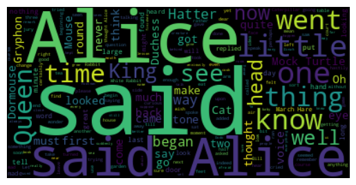
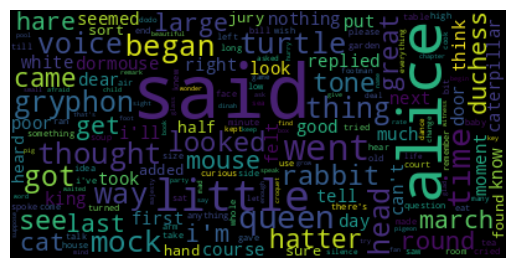
(200, 400, 3)

WordCloud 객체의 generate메서드에 입력으로 문서를 넘겨주면 알아서 토큰화 등의 작업을 합니다. 그러나 이전에 토큰화 및 불용어 제거, 품사 태깅 및 특정 품사만 걸러내기 등의 작업을 했었는데, 이를 활용할 수 있는 방법이 없을까요?

generate_form_frequencies() 메서드를 이용하면 됩니다.

wordcloud = WordCloud(max_font_size=60).generate_from_frequencies(alice_word_count)

plt.figure()
plt.axis('off')
plt.imshow(wordcloud, interpolation='bilinear')
plt.show()

실행 결과

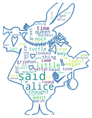
여기에 살짝 멋을 부려볼까요?

배경이 되는 이미지는 Pixabay로부터 입수된 Clker-Free-Vector-Images님의 이미지 입니다.

import numpy as np
from PIL import Image

alice_mask = np.array(Image.open("alice-in-wonderland.png"))

wc = WordCloud(background_color='white',
               max_words=50,
               mask=alice_mask,
               contour_width=3,
               contour_color='steelblue')

wc.generate_from_frequencies(alice_word_count)

wc.to_file("alice.png")

plt.figure()
plt.axis('off')
plt.imshow(wc, interpolation='bilinear')
plt.show()

실행 결과

3.3 한국어 문서에 대한 그래프와 워드 클라우드

한글 워드 클라우드를 그리기 위해 먼저 예제로 사용할 텍스트를 불러옵시다. KoNLPy는 형태소 분석기도 제공하지만, 실습을 위해 사용할 말뭉치도 제공합니다. 그중 하나가 대한민국 헌법입니다. 헌법 텍스트를 불러오고 타입과 문자 수, 텍스트 일부분을 한 번 확인해봅시다.

from konlpy.corpus import kolaw
const_doc = kolaw.open('constitution.txt').read()

print(type(const_doc))
print(len(const_doc))
print(const_doc[:600])

실행 결과

<class 'str'>
18884
대한민국헌법

유구한 역사와 전통에 빛나는 우리 대한국민은 3·1운동으로 건립된 대한민국임시정부의 법통과 불의에 항거한 4·19민주이념을 계승하고, 조국의 민주개혁과 평화적 통일의 사명에 입각하여 정의·인도와 동포애로써 민족의 단결을 공고히 하고, 모든 사회적 폐습과 불의를 타파하며, 자율과 조화를 바탕으로 자유민주적 기본질서를 더욱 확고히 하여 정치·경제·사회·문화의 모든 영역에 있어서 각인의 기회를 균등히 하고, 능력을 최고도로 발휘하게 하며, 자유와 권리에 따르는 책임과 의무를 완수하게 하여, 안으로는 국민생활의 균등한 향상을 기하고 밖으로는 항구적인 세계평화와 인류공영에 이바지함으로써 우리들과 우리들의 자손의 안전과 자유와 행복을 영원히 확보할 것을 다짐하면서 1948년 7월 12일에 제정되고 8차에 걸쳐 개정된 헌법을 이제 국회의 의결을 거쳐 국민투표에 의하여 개정한다.

       제1장 총강
  제1조 ① 대한민국은 민주공화국이다.
②대한민국의 주권은 국민에게 있고, 모든 권력은 국민으로부터 나온다.
  제2조 ① 대한민국의 국민이 되는 요건은 법률로 정한다.
②국가는 법률이 정하는 바에 의하여 재외국민을 보호할 의무를 진다.
  제3조 대한민

대한민국 헌법은 총 18,884로 구성되어있습니다.

이제 형태소 분석을 실시하고 분석해봅시다.

from konlpy.tag import Okt
t = Okt()
tokens_const = t.morphs(const_doc)

print("Nbr of tokens:", len(tokens_const))
print("Tokens sample:")
print(tokens_const[:100])

실행 결과

Nbr of tokens: 8796
Tokens sample:
['대한민국', '헌법', '\n\n', '유구', '한', '역사', '와', '전통', '에', '빛나는', '우리', '대', '한', '국민', '은', '3', '·', '1', '운동', '으로', '건립', '된', '대한민국', '임시정부', '의', '법', '통과', '불의', '에', '항거', '한', '4', '·', '19', '민주', '이념', '을', '계승', '하고', ',', '조국', '의', '민주', '개혁', '과', '평화', '적', '통일', '의', '사명', '에', '입', '각하', '여', '정의', '·', '인도', '와', '동포', '애', '로써', '민족', '의', '단결', '을', '공고', '히', '하고', ',', '모든', '사회', '적', '폐습', '과', '불의', '를', '타파', '하며', ',', '자율', '과', '조화', '를', '바탕', '으로', '자유민주', '적', '기', '본', '질서', '를', '더욱', '확고히', '하여', '정치', '·', '경제', '·', '사회', '·']

이렇게 보면 기호나 숫자, 그리고 조사 등은 의미가 없는 것으로 보입니다. 명사만 추출해봅시다.

tokens_const = t.nouns(const_doc)

print("Nbr of tokens:", len(tokens_const))
print("Tokens sample:")
print(tokens_const[:100])

실행 결과

Nbr of tokens: 3882
Tokens sample:
['대한민국', '헌법', '유구', '역사', '전통', '우리', '국민', '운동', '건립', '대한민국', '임시정부', '법', '통과', '불의', '항거', '민주', '이념', '계승', '조국', '민주', '개혁', '평화', '통일', '사명', '입', '각하', '정의', '인도', '동포', '애', '로써', '민족', '단결', '공고', '모든', '사회', '폐습', '불의', '타파', '자율', '조화', '바탕', '자유민주', '질서', '더욱', '정치', '경제', '사회', '문화', '모든', '영역', '각인', '기회', '능력', '최고', '도로', '발휘', '자유', '권리', '책임', '의무', '완수', '안', '국민', '생활', '향상', '기하', '밖', '항구', '세계', '평화', '인류', '공영', '이바지', '함', '우리', '우리', '자손', '안전', '자유', '행복', '확보', '것', '다짐', '제정', '차', '개정', '헌법', '이제', '국회', '의결', '국민투표', '개정', '제', '장', '강', '제', '대한민국', '민주공화국', '대한민국']

앞선 결과보다는 나아보이지만 무언가 아쉬운 부분이 남아있습니다. 한 글자 명사들, '것', '애' 등등은 의미가 없어보입니다. 한 글자로 되어있는 명사를 삭제하고 결과를 살펴봅시다.

tokens_const= [token for token in tokens_const if len(token) > 1]

print("Nbr of tokens:", len(tokens_const))
print("Tokens sample:")
print(tokens_const[:100])

실행 결과

Nbr of tokens: 3013
Tokens sample:
['대한민국', '헌법', '유구', '역사', '전통', '우리', '국민', '운동', '건립', '대한민국', '임시정부', '통과', '불의', '항거', '민주', '이념', '계승', '조국', '민주', '개혁', '평화', '통일', '사명', '각하', '정의', '인도', '동포', '로써', '민족', '단결', '공고', '모든', '사회', '폐습', '불의', '타파', '자율', '조화', '바탕', '자유민주', '질서', '더욱', '정치', '경제', '사회', '문화', '모든', '영역', '각인', '기회', '능력', '최고', '도로', '발휘', '자유', '권리', '책임', '의무', '완수', '국민', '생활', '향상', '기하', '항구', '세계', '평화', '인류', '공영', '이바지', '우리', '우리', '자손', '안전', '자유', '행복', '확보', '다짐', '제정', '개정', '헌법', '이제', '국회', '의결', '국민투표', '개정', '대한민국', '민주공화국', '대한민국', '주권', '국민', '모든', '권력', '국민', '대한민국', '국민', '요건', '법률', '국가', '법률', '재외국민']

이 정도면 어느 정도 만족스럽다고 할 수 있습니다.

이제 수평 막대 그래프를 그려봅시다. 단, 여기서는 한글 폰트를 지정해야 한다고 한다.

wsl 환경에서 폰트 지정하기
WSL에서 Windows font 사용하기 (feat. matplotlib font)
위 블로그를 참고하여 진행하였다.

import matplotlib.pyplot as plt
plt.rc('font', family='NanumGothic')

const_cnt = {}
for word in tokens_const:
    const_cnt[word] = const_cnt.get(word, 0) + 1

def word_graph(cnt, max_words=10) :
    sorted_w = sorted(cnt.items(), key=lambda kv: kv[1])
    print(sorted_w[-max_words:])
    n, w = zip(*sorted_w[-max_words:])

    plt.barh(n, w)
    plt.show()

word_graph(const_cnt, max_words=20)

실행 결과

[('조직', 18), ('국회의원', 18), ('임기', 18), ('직무', 19), ('국무총리', 19), ('자유', 20), ('정부', 20), ('선거', 20), ('임명', 20), ('권리', 21), ('의원', 21), ('사항', 23), ('기타', 26), ('모든', 37), ('헌법', 53), ('국민', 61), ('국회', 68), ('국가', 73), ('대통령', 83), ('법률', 127)]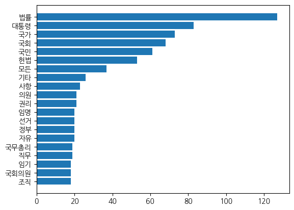

이제 워드 클라우드를 그려봅시다.

wsl에서 폰트 지정하기
https://velog.io/@2hey9/final-project-airflow%EB%A5%BC-%ED%99%9C%EC%9A%A9%ED%95%9C-wordcloud-%EC%83%9D%EC%84%B12-python-%ED%8C%8C%EC%9D%BC-%EC%9E%91%EC%84%B1-%EB%B0%8F-WSL%EC%97%90%EC%84%9C-%EC%8B%A4%ED%96%89-%ED%99%95%EC%9D%B8
위 블로그를 참고하여 진행했다.

font_path = "./NanumGothic.ttf"
wordcloud = WordCloud(font_path=font_path).generate(const_doc)

plt.axis("off")
plt.imshow(wordcloud, interpolation='bilinear')
plt.show()

실행 결과

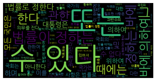
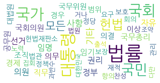
자동으로 토큰화 및 빈도분석을 해주다보니 만족스러운 결과가 나오지 않았습니다. 형태소 분석이 된 값으로 다시 실습을 진행해봅시다.

이번에는 워드 클라우드를 살짝 더 꾸몄습니다.

wordcloud = WordCloud(
    font_path=font_path,
    max_font_size=100,
    width=800,
    height=400,
    background_color='white',
    max_words=50
)

wordcloud.generate_from_frequencies(const_cnt)

wordcloud.to_file('const.png')

plt.axis("off")
plt.imshow(wordcloud, interpolation='bilinear')
plt.show()

실습 결과