Credit Card Fraud Detection
주피터에서 실제 데이터를 이용하여 이상거래 데이터셋에 대한 EDA 작업을 해보자!!
데이터 출처 : https://www.kaggle.com/mlg-ulb/creditcardfraud
1. 데이터 불러오기
데이터 출처 : https://www.kaggle.com/mlg-ulb/creditcardfraud
credit_card = pd.read_csv("../Data/Fraud Detection/creditcard.csv")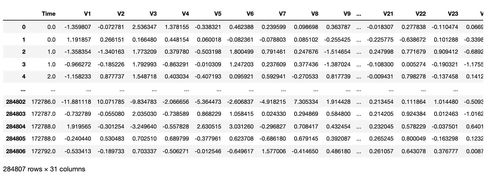
2. 데이터 Exploration

-
거래 금액(Amount), 거래시간 외에, 28개의 특성 존재
-
class를 제외한 모든 feature 데이터 타입은 float64
-
class는 이상 거래이면 1, 정상 거래이면 0
-
time은 초단위 기록
2-1. 정상거래 vs. 비정상거래 데이터 확인
plt.figure(figsize=(10, 5))
sns.countplot(x='Class', data = credit_card)
plt.title("Class Distribution \n (0= Geuine | 1 = Fraudulent)")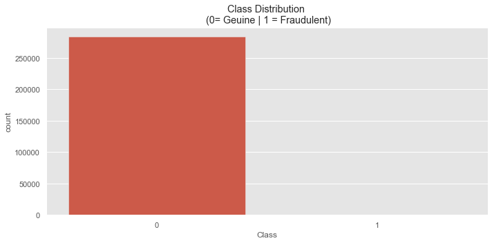
- 정상거래와, 비정상거래의 수가 상당히 imbalanced 된 것을 확인 할 수 있다.
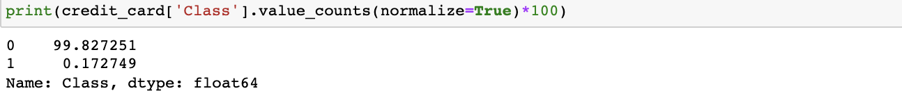
- 정상거래와, 비정상거래의 수를 정규화 하였을 경우, 이상거래로 탐지된 데이터는 반올림 해서 대략 0.2% 밖에 없다는 것을 확인할 수 있다.
5-2 데이터 분리(학습용 vs 훈련용)
test_train dataset으로 나누기 위해선 데이터가 심하게 정상거래 쪽으로 치울어져 있기 때문에, stratify 옵션을 사용하여 train_test_split에 비정상거래 데이터도 포함되도록 해야한다.
train, test = train_test_split(credit_card, test_size = 0.2, shuffle=True, stratify=credit_card['Class'])
print("Train Shape: {} \nTest Shape: {}".format(train.shape, test.shape))
Train Shape: (227845, 31)
Test Shape: (56962, 31)print("Train: \n")
print(train['Class'].value_counts(normalize=True) * 100, '\n')
print("Test: \n")
print(test['Class'].value_counts(normalize=True) * 100, '\n')정규화 처리후 결과:
Train:

0    99.827075
1     0.172925
Name: Class, dtype: float64

Test:

0    99.827955
1     0.172045
Name: Class, dtype: float64
2-2. 시간 vs 거래금액 관계
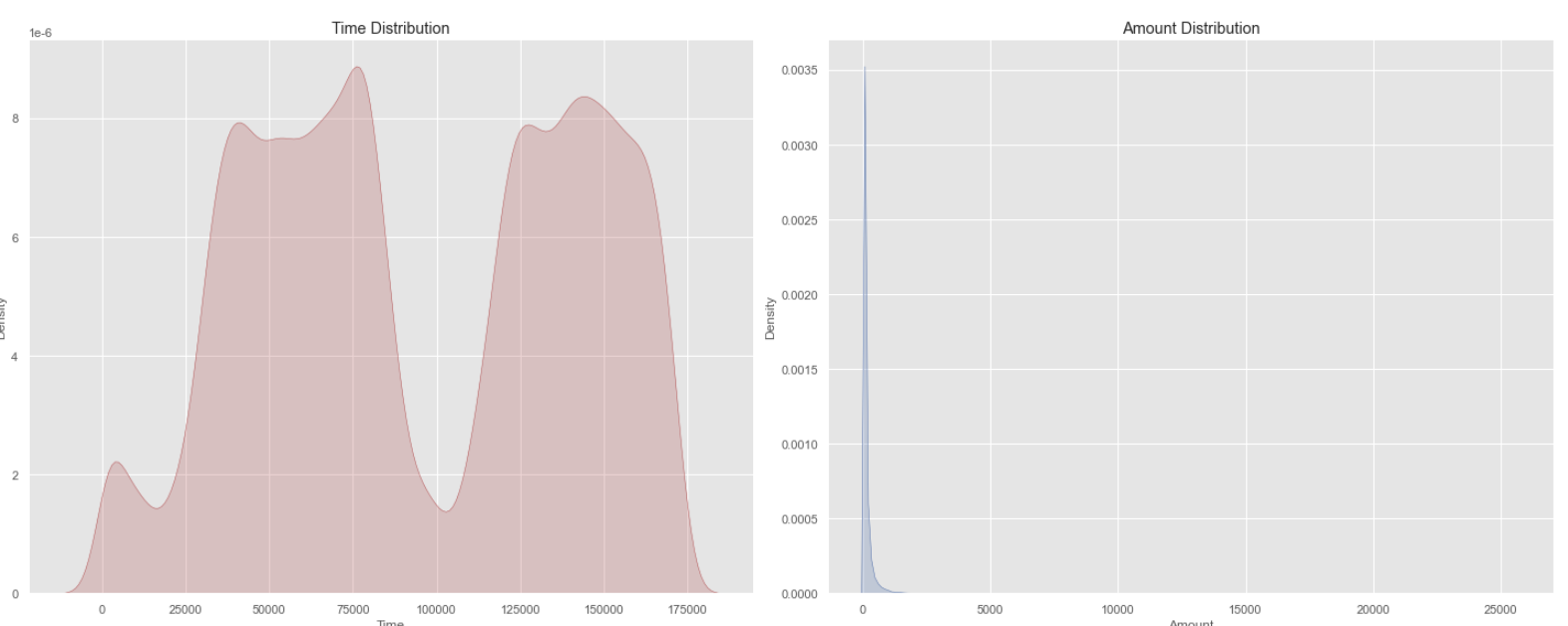
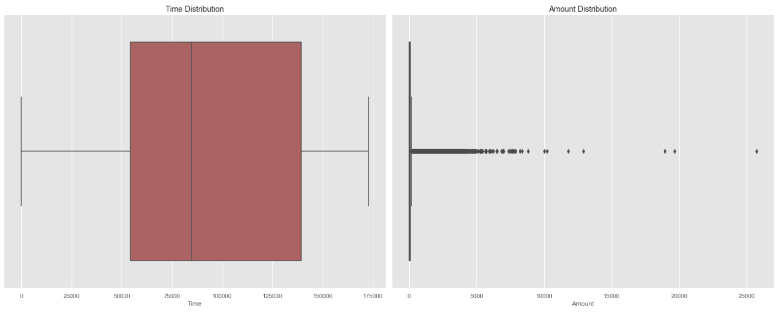
- 신용 거래는 전체적인 시간에 발생하는 것을 확인할 수 있으며, 대부분 0~100 사이의 금액을 사용하는 것을 파악할 수 있다.
2-3 Anonymized Features 파악
anon_df = train.drop(['Time', 'Amount', 'Class'], axis = 1)

fig, axs = plt.subplots(4, 7, figsize=(15, 15))

for col in range(len(anon_df.columns)):
    column = anon_df.columns[col]
    plt.subplot(4, 7, col+1)
    sns.boxplot(data=anon_df[column])
    plt.title(str(column))
    plt.xticks([]) # Remove X ticks

plt.tight_layout();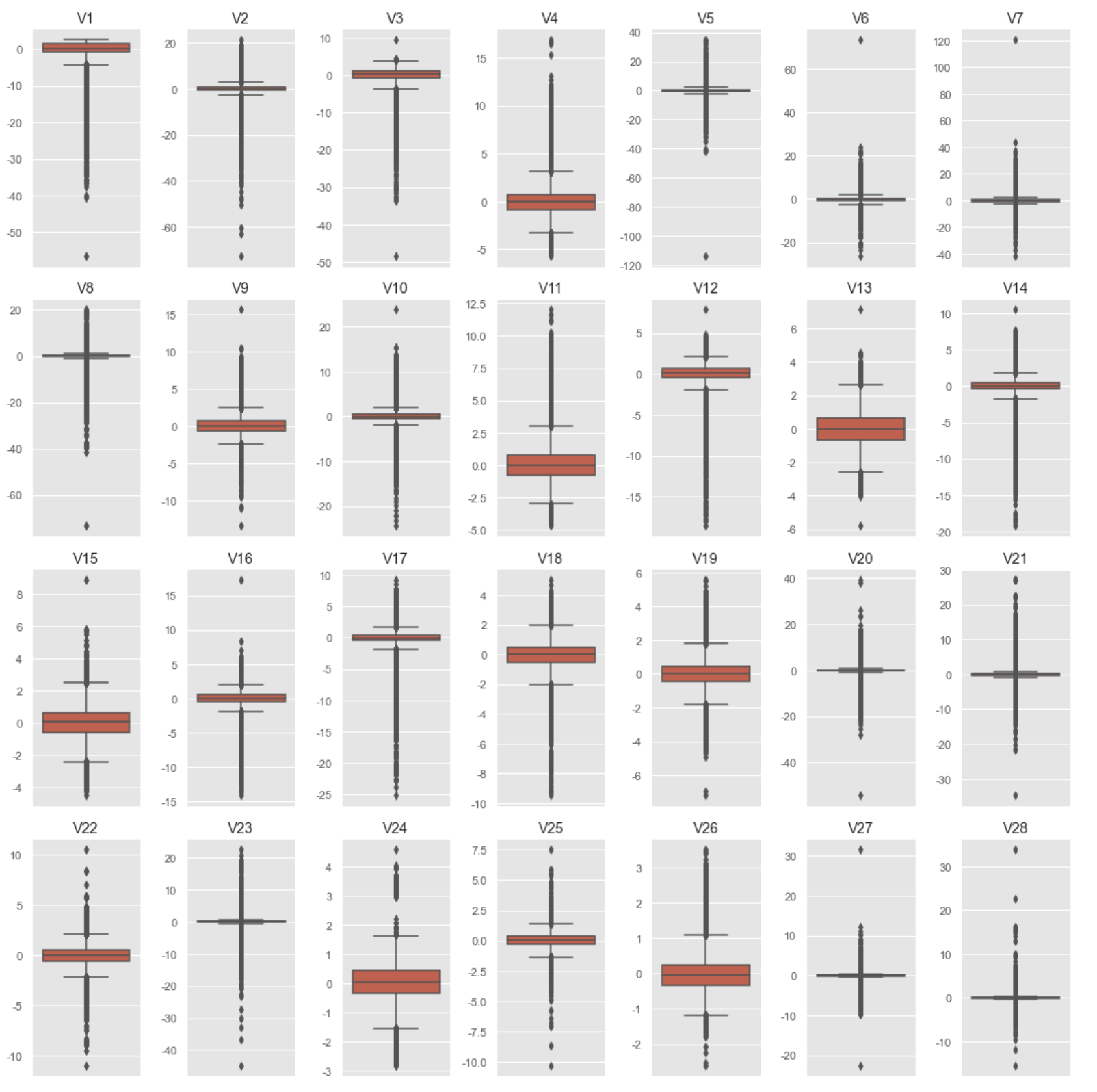
- 모든 항목들이 대부분 0을 중심으로 두고 있다는 것을 알 수 있다.
- 모든 항목들의 데이터가 각각 다 다르기 때문에, scale을 적용해줄 필요가 있다.
2-4 Anonymized Feature에 Feature Scaling 적용
X_train = train.drop('Class', axis=1)
y_train = train['Class']
X_test = test.drop('Class', axis=1)
y_test = test['Class']

print("X_train shape: {} \ny_train shape: {}\nX_test shape: {}\ny_test shape: {}"\
      .format(X_train.shape, y_train.shape, X_test.shape, y_test.shape))

robust_scaler = RobustScaler()
X_train = robust_scaler.fit_transform(X_train)
X_test = robust_scaler.transform(X_test)
X_train shape: (227845, 30)
y_train shape: (227845,)
X_test shape: (56962, 30)
y_test shape: (56962,)
3. Data Imbalance 문제
현재 신용거래 데이터에서, 비정상거래 감지 데이터가 정상거래 데이터에 비해 현저히 낮다. 그래서 학습을 시킬 경우에도, 비정상거래 감지 데이터셋이 충분하지 않기 때문에, 학습이 제대로 되지 않을 것이다.
이 같은 문제를 해결하기 위해 기본적으로 1. Undersampling 방법과 2. Oversampling-SMOTE 방법을 사용할 수 있다.
-
Undersampling은 전체 데이터셋을 충분하지 않은 클래스의 데이터셋 기준으로 random sampling하는 것이다.
하지만, 이 방법의 문제는 많은 데이터의 양을 버리게 된다는 것이다. -
Oversampling SMOTE은 Synthetic Minority Oversampling Technique의 준말이며, Data Imbalance문제를 해결할 때 가장 많이 쓰이는 방법이다.
이 방법은 K-NN 기법을 이용하여 소수 클래스 데이터와 그 데이터에서 가장 가까운 k개의 소수 클래스 데이터 중 무작위로 선택된 데이터 사이의 직선상에 가상의 소수 클래스 데이터를 만드는 방법이다
3-1 Synthetic Minority Oversampling Technique (SMOTE) 적용
smote_upsampler = SMOTE(sampling_strategy='minority', k_neighbors=5, n_jobs=-1)
X_train_upsample, y_train_upsample = smote_upsampler.fit_resample(X_train, y_train)
print('After upsampling: \nX_train shape: {} \ny_train shape: {}'.format(X_train_upsample.shape, y_train_upsample.shape))
After upsampling:
X_train shape: (454902, 30)
y_train shape: (454902,)plt.figure(figsize=(5,5))
plt.title('Distribution of Target Variables After Upsampling \n(0 = Genuine | 1 = Fraudulent)')
sns.countplot(y_train_upsample);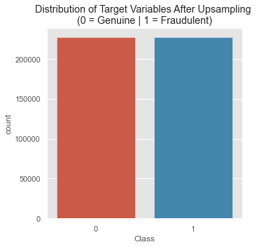
3-2 Cross-Validation with SMOTE
비정상거래 데이터의 수를 함부로?? 생성해냈기 때문에, 이에 대한 합법성을 확인 하기 위해 Cross Validation Check를 해주면 좋다.
def smote_cv(model, X, y, parms=None, cv=5, random_state=13):

  smote_cv = StratifiedKFold(n_splits=cv, shuffle=True, random_state=random_state)
  smote = SMOTE(sampling_strategy='minority', k_neighbors=5)

  # Ensure data is in dataframe
  X = pd.DataFrame(X)
  y = pd.DataFrame(y)

  precision_scores = []
  f1_scores = []
  recall_scores = []

  for train_index, valid_index in smote_cv.split(X, y):
    # Use indices to split data
    X_train = X.iloc[train_index]
    y_train = y.iloc[train_index]
    X_valid = X.iloc[valid_index]
    y_valid = y.iloc[valid_index]

    # Apply SMOTE, but only to the training fold
    X_train_smote, y_train_smote = smote.fit_resample(X_train, y_train)

    # Fit model with new data
    model_smote = model.fit(
        X_train_smote, y_train_smote
    )

    # Make validation predictions
    y_pred = model_smote.predict(X_valid)

    #Score model using upsampled train data and original validation data
    f1 = f1_score(y_valid, y_pred)
    recall = recall_score(y_valid, y_pred)
    precision = precision_score(y_valid, y_pred)

    f1_scores.append(f1)
    recall_scores.append(recall)
    precision_scores.append(precision)

  return {'f1': f1_scores, 'recall': recall_scores, 'precision': precision_scores}
4 Rogistic Regression Model 적용
%%time
cv_pipeline(log_clf, output_type='print')
적용 결과:
Model: LogisticRegression
F1 score:0.1114
Precision: 0.0594
Recall: 0.9035
CPU times: user 1min 47s, sys: 26.5 s, total: 2min 14s
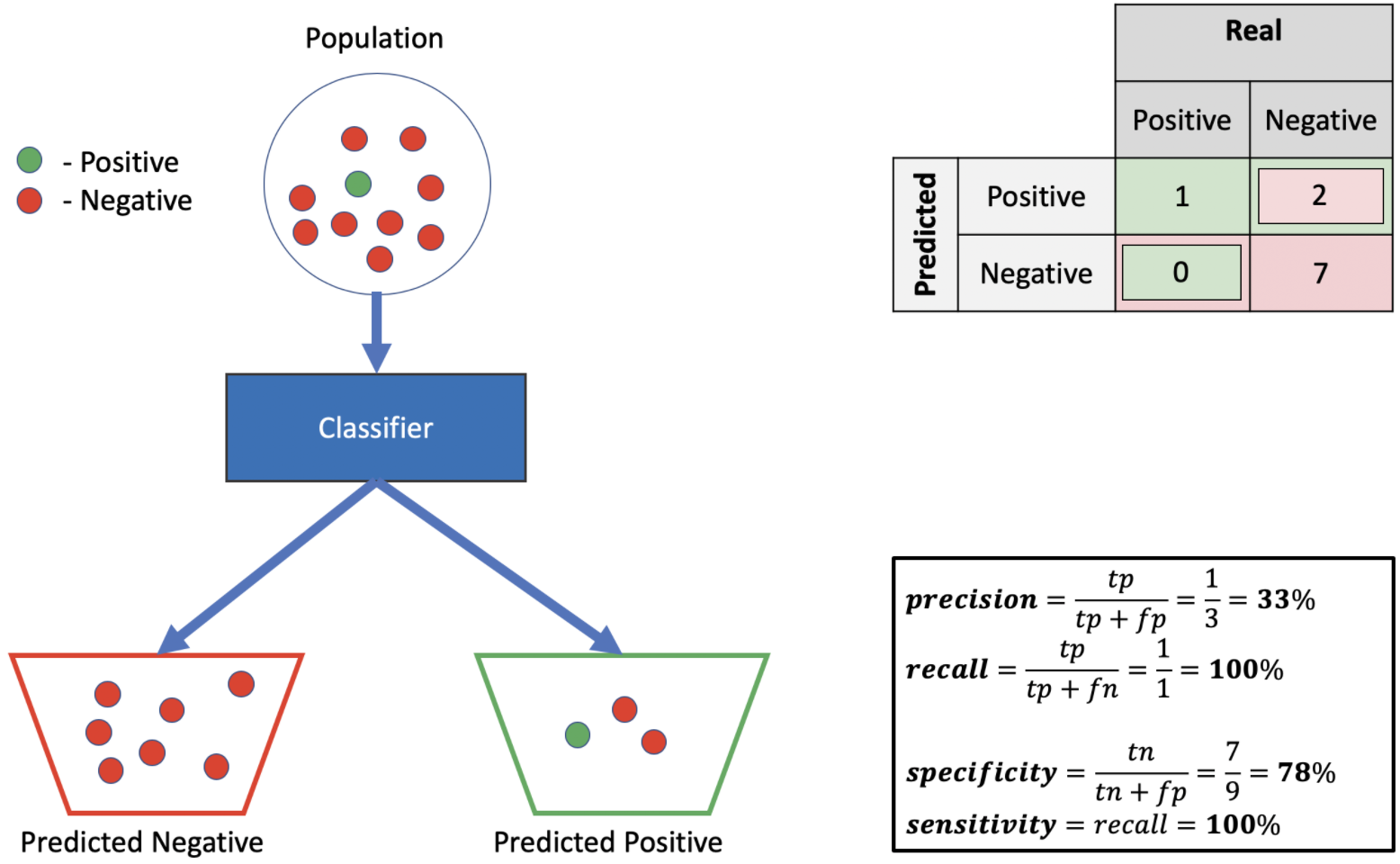
Wall time: 17.7 sPrecision - Recall
현재 이 데이터셋은 imbalanced 되어있기 때문에 precision과 recall 값을 확인하며 분류 예측모델의 평가를 확인해야 한다.
5. 다른 분류기로 결과 확인
| Model | f1_score | precision | recall | time | |
|---|---|---|---|---|---|
| 3 | LGBMClassifier | 0.647125 | 0.531362 | 0.832457 | 9.292184 |
| 2 | XGBClassifier | 0.420426 | 0.279313 | 0.865498 | 90.975678 |
| 1 | RandomForestClassifier | 0.342974 | 0.216378 | 0.862934 | 76.66814 |
| 0 | LogisticRegression | 0.11143 | 0.059406 | 0.903473 | 17.658714 |
6-1 LGBM
LGBM분류기의 학습 결과는 과적합일 가능성이 높다. 그래서 learning curve를 확인하며 parameter를 조정해줘야 한다.
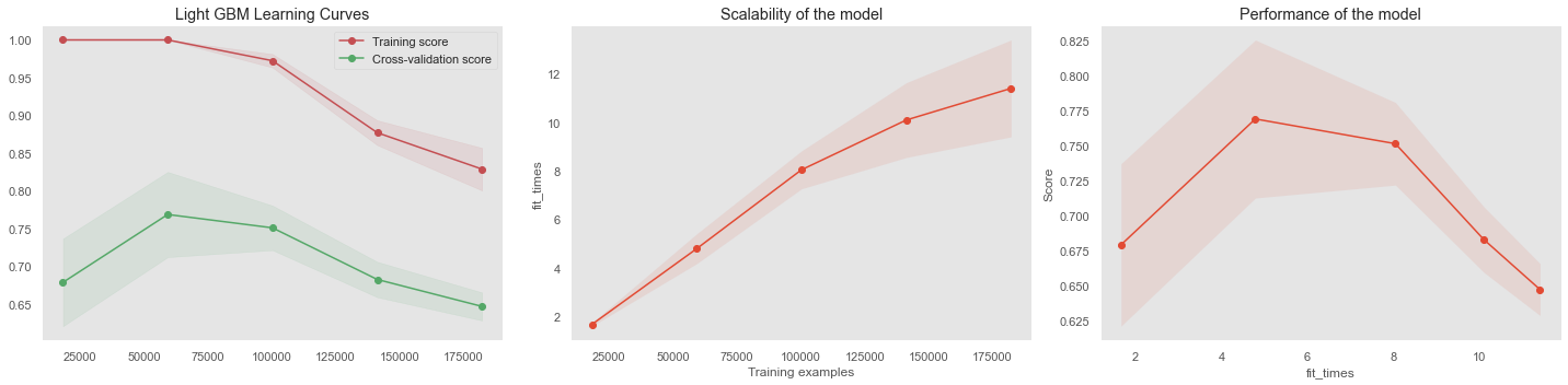
학습을 시킬 수록 validation score와 training score가 떨어지는 지면 학습모델이 과적합이 발생했다고 판단해도 된다.
이것을 해결하기 위해, hyperparamer optimization을 해주어야 한다.
hyperparameter찾은 후, 결과:

start = time.time()
cv_pipeline(lgb_pipeline, output_type='print')
print('Time: {:.2f}'.format(time.time()-start))
Model: Pipeline
F1 score:0.8035
Precision: 0.8076
Recall: 0.7995
Time: 14.917. Gradient Boosting Model 평가
7-1 LightGBM
model = LGBMClassifier(
    tree_learner = 'serial',
    # More operational parameters
    n_jobs = -1, force_col_wise= True, verbose=0,
    # Model parameters
    n_estimators = 100,
    num_leaves = 255, learning_rate = 0.1,
    subsample = 0.7,
    )
model.fit(X_train_upsample, y_train_upsample)
y_pred = model.predict(X_test)
plot_confusion(y_test, y_pred)
7-2 XGBoost
xgb_params = {
    'clf__col_samply_by_tree': 1.3524460165118497,
    'clf__gamma': 73,
    'clf__learning_rate': 0.5318304572904284,
    'clf__max_depth': 4,
    'clf__min_child_weight': 1,
    'clf__n_estimators': 139,
    'clf__reg_alpha': 0.7561010481304831
              }

model = XGBClassifier(**xgb_params)
model.fit(X_train_upsample, y_train_upsample)
y_pred = model.predict(X_test)
plot_confusion(y_test, y_pred)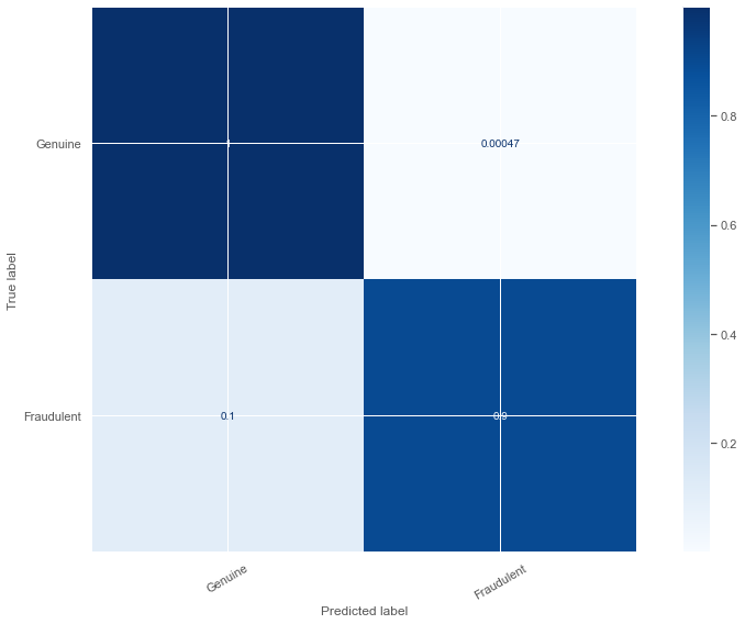
10. 결과
Kaggle에서 제공된 신용카드 거래 데이터를 활용하여 EDA작업 및, 이상 거래 탐지 모델을 설계해보았다.
이상 거래의 경우, heavily imbalanced 했었기 때문에, SMOTE 기법을 사용하여 upsampling해주어야 했다.
XGBoost와 LightGBM에서의 hyperparameter 를 찾을 경우, randomized search 기법을 활용하여야 최상의 best_fit 결과를 가져올 수 있었다.
하지만, randomized_search기법으로 큰 범위 파라미터를 확인해본다면, 다소 시간이 아주 오래 걸린다는 단점이 있다.
XGBoost Model의 최종 결과로는 이상 거래 데이터 중 88%를 감지 할 수 있었으며, 정상적인 거래는 99% 예측할 수 있었다.
