<논문>[arXiv] Denoising Diffusion Implicit Models
<참고자료>[tistory] DDIM : Denoising Diffusion Implicit Models [page] [논문리뷰] DDIM : Denoising Diffusion Implicit Model
DDIM은 DDPMs의 후속 논문이다. DDPMs의 단점인 '느린 Sampling 속도'를 해결하고자 새로운 Sampling 방안을 제시하였다. 이 포스팅은 DDPMs를 안다는 전제 하에 진행될 것이므로 DDPMs 를 먼저 알고 오는 것을 권장한다.
1. Introduction
기존의 이미지 생성 모델인 VAE는 다양한 이미지를 생성할 수 있지만 quality가 낮았고, GAN은 높은 quality의 이미지를 생성할 수 있지만 다양성이 낮았다. 이와 달리 DDPMs의 diffusion model은 높은 quality의 이미지를 다양하게 생성할 수 있었지만, Sampling 속도가 느리다는 단점이 있었다. diffusion model의 구조 상, Pure Gaussian Noise에 T ( = 1000 ) T(=1000) T ( = 1 0 0 0 )
DDIM은 non-Markovian diffusion process를 활용하여 DDPMs에서의 Sampling 속도를 10배 이상 향상시킨다. 또한 consistency를 향상시켜, 비슷한 위치에서 x T \mathbf{x}_T x T
시작하기에 앞서, DDIM에서 사용하는 α t \alpha_t α t α t = 1 − β t \alpha_t = 1-\beta_t α t = 1 − β t α t = ∏ i = 1 T ( 1 − β t ) \alpha_t = \prod_{i=1}^T(1-\beta_t) α t = ∏ i = 1 T ( 1 − β t ) α ˉ t \bar{\alpha}_t α ˉ t α t \alpha_t α t DDPMs 기준의 α t \alpha_t α t
2. 개요
DDPMs의 느린 Sampling 속도는 무엇 때문일까? DDIM은 Markov Chain을 원인으로 보았다. 이미지를 Sampling 하는 데 T ( = 1000 ) T(=1000) T ( = 1 0 0 0 ) 몇 단계씩 건너뛰며 Sampling 속도를 높이자 는 것이 DDIM의 주장이다. 이를 위해 non-Markovian Forward process와 non-Markovian Reverse process를 제안하고, Reverse process가 T ( = 1000 ) T(=1000) T ( = 1 0 0 0 )
process가 바뀌면 Loss function이 바뀌는 것이 일반적인데, DDIM의 핵심 중 하나는 Loss function이 바뀌었음에도 불구하고 최적해의 위치는 바뀌지 않는다 는 것이다. 즉 파라미터 θ \theta θ
3. Non-Markovian process
우선 DDPMs에서의 Loss function을 다시 떠올려보자.
L s i m p l e ( θ ) = E t , x 0 , ϵ [ ( ϵ − ϵ θ ( x t , t ) ) 2 ] L_{simple}(\theta) = \mathrm{E}_{{t}, \mathbf{x}_0, \epsilon} \bigg[ (\epsilon - \epsilon_{\theta}(\mathbf{x}_t, t))^2 \bigg] L s i m p l e ( θ ) = E t , x 0 , ϵ [ ( ϵ − ϵ θ ( x t , t ) ) 2 ] Simple Loss function은 기존의 KL Divergence의 합으로부터, t t t ( = β t 2 2 σ t 2 α t ( 1 − α ˉ t ) ) (={\beta_t^2 \over 2\sigma_t^2\alpha_t (1-\bar{\alpha}_t)}) ( = 2 σ t 2 α t ( 1 − α ˉ t ) β t 2 )
L γ ( ϵ θ ) ≔ ∑ t = 1 T γ t E x 0 ∼ q ( x 0 ) , ϵ t ∼ N ( 0 , I ) [ ∣ ∣ ϵ θ ( t ) ( x t , t ) − ϵ t ∣ ∣ 2 2 ] L_\gamma(\epsilon_\theta) \coloneqq \sum_{t=1}^T \gamma_t \mathrm{E}_{\mathbf{x}_0 \sim q(\mathbf{x}_0),\epsilon_t \sim N(0, I)} \bigg[ ||\epsilon_\theta^{(t)}(\mathbf{x}_t, t) - \epsilon_t||_2^2 \bigg] L γ ( ϵ θ ) : = t = 1 ∑ T γ t E x 0 ∼ q ( x 0 ) , ϵ t ∼ N ( 0 , I ) [ ∣ ∣ ϵ θ ( t ) ( x t , t ) − ϵ t ∣ ∣ 2 2 ] DDPMs는 본래 γ t = β t 2 2 σ t 2 α t ( 1 − α ˉ t ) \gamma_t ={\beta_t^2 \over 2\sigma_t^2\alpha_t (1-\bar{\alpha}_t)} γ t = 2 σ t 2 α t ( 1 − α ˉ t ) β t 2 γ t = 1 \gamma_t=1 γ t = 1 γ t \gamma_t γ t
DDIM에서 중요하게 본 포인트는 Loss function이 marginal distribution인 q ( x t ∣ x 0 ) q(\mathbf{x}_t~|~\mathbf{x}_0) q ( x t ∣ x 0 ) 되고, joint distribution인 q ( x 1 : T ∣ x 0 ) q(\mathbf{x}_{1:T}~|~\mathbf{x}_0) q ( x 1 : T ∣ x 0 ) [1] 즉, marginal distribution만 유지한다면 joint distribution은 무엇이 와도 상관없다고 해석하여, 같은 marginal distribution을 갖는 다른 process를 고려한다. 그 중, Markov process를 다룬 DDPMs와 달리 non-Markov process를 정의할 것이다.
3-1. Definition
위에서 언급한 바와 같이 non-Markovian process q σ q_\sigma q σ q σ ( x t ∣ x 0 ) = N ( x t ; α ˉ t x 0 , ( 1 − α ˉ t ) I ) q_\sigma(\mathbf{x}_t~|~\mathbf{x}_0) = N(\mathbf{x}_t~;~\sqrt{\bar{\alpha}_t}\mathbf{x}_0, (1-\bar{\alpha}_t)I) q σ ( x t ∣ x 0 ) = N ( x t ; α ˉ t x 0 , ( 1 − α ˉ t ) I ) q σ q_\sigma q σ
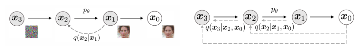
q σ ( x 1 : T ∣ x 0 ) ≔ q σ ( x 1 ∣ x 0 ) ∏ t = 2 T q σ ( x t ∣ x t − 1 , x 0 ) q_\sigma(\mathbf{x}_{1:T}~|~\mathbf{x}_0) \coloneqq q_\sigma(\mathbf{x}_1~|~\mathbf{x}_0) \prod_{t=2}^T q_\sigma(\mathbf{x}_t~|~\mathbf{x}_{t-1}, \mathbf{x}_0) q σ ( x 1 : T ∣ x 0 ) : = q σ ( x 1 ∣ x 0 ) t = 2 ∏ T q σ ( x t ∣ x t − 1 , x 0 ) 위의 식을 잘 살펴보면, x 0 \mathbf{x}_0 x 0 x 1 \mathbf{x}_1 x 1 ( = q σ ( x 1 ∣ x 0 ) ) (=q_\sigma(\mathbf{x}_1~|~\mathbf{x}_0)) ( = q σ ( x 1 ∣ x 0 ) ) q σ ( x t ∣ x t − 1 , x 0 ) q_\sigma(\mathbf{x}_t~|~\mathbf{x}_{t-1}, \mathbf{x}_0) q σ ( x t ∣ x t − 1 , x 0 ) x 2 \mathbf{x}_2 x 2 x 3 \mathbf{x}_3 x 3 ⋯ \cdots ⋯ x T \mathbf{x}_T x T DDIM(오른쪽)은 직전과 처음 이미지를 참고하는 것이다.
q σ ( x 1 : T ∣ x 0 ) = q σ ( x 1 ∣ x 0 ) ∏ t = 2 T q σ ( x t ∣ x t − 1 , x 0 ) = q σ ( x 1 ∣ x 0 ) ∏ t = 2 T q σ ( x t − 1 ∣ x t , x 0 ) q σ ( x t ∣ x 0 ) q σ ( x t − 1 ∣ x 0 ) = q σ ( x T ∣ x 0 ) ∏ t = 2 T q σ ( x t − 1 ∣ x t , x 0 ) \begin{aligned} q_\sigma(\mathbf{x}_{1:T}~|~\mathbf{x}_0) &= q_\sigma(\mathbf{x}_1~|~\mathbf{x}_0) \prod_{t=2}^T q_\sigma(\mathbf{x}_t~|~\mathbf{x}_{t-1}, \mathbf{x}_0) \\ &= q_\sigma(\mathbf{x}_1~|~\mathbf{x}_0) \prod_{t=2}^T {q_\sigma(\mathbf{x}_{t-1}~|~\mathbf{x}_t,\mathbf{x}_0)~q_\sigma(\mathbf{x}_t~|~\mathbf{x}_0) \over q_\sigma(\mathbf{x}_{t-1}~|~\mathbf{x}_0)} \\ &= q_\sigma(\mathbf{x}_T~|~\mathbf{x}_0) \prod_{t=2}^T q_\sigma(\mathbf{x}_{t-1}~|~\mathbf{x}_t,\mathbf{x}_0) \end{aligned} q σ ( x 1 : T ∣ x 0 ) = q σ ( x 1 ∣ x 0 ) t = 2 ∏ T q σ ( x t ∣ x t − 1 , x 0 ) = q σ ( x 1 ∣ x 0 ) t = 2 ∏ T q σ ( x t − 1 ∣ x 0 ) q σ ( x t − 1 ∣ x t , x 0 ) q σ ( x t ∣ x 0 ) = q σ ( x T ∣ x 0 ) t = 2 ∏ T q σ ( x t − 1 ∣ x t , x 0 ) 이다. 어떠한 forward process든 pure Gaussian Noise를 목표로 함은 같으므로
q σ ( x T ∣ x 0 ) ≔ N ( α ˉ T x 0 , ( 1 − α ˉ T ) I ) q_\sigma(\mathbf{x}_T~|~\mathbf{x}_0) \coloneqq N(\sqrt{\bar{\alpha}_T}\mathbf{x}_0, (1-\bar{\alpha}_T)I) q σ ( x T ∣ x 0 ) : = N ( α ˉ T x 0 , ( 1 − α ˉ T ) I ) 로 정의할 수 있다.t > 1 t>1 t > 1
q σ ( x t − 1 ∣ x t , x 0 ) = N ( α ˉ t − 1 x 0 + 1 − α ˉ t − 1 − σ t 2 ⋅ x t − α ˉ t x 0 1 − α ˉ t , σ t 2 I ) q_\sigma(\mathbf{x}_{t-1}~|~\mathbf{x}_t, \mathbf{x}_0) = N(\sqrt{\bar{\alpha}_{t-1}}\mathbf{x}_0 + \sqrt{1-\bar{\alpha}_{t-1}-\sigma_t^2} \cdot {\mathbf{x}_t-\sqrt{\bar{\alpha}_t}\mathbf{x}_0 \over \sqrt{1-\bar{\alpha}_t}}, \sigma_t^2I) q σ ( x t − 1 ∣ x t , x 0 ) = N ( α ˉ t − 1 x 0 + 1 − α ˉ t − 1 − σ t 2 ⋅ 1 − α ˉ t x t − α ˉ t x 0 , σ t 2 I ) 라 정의하자. 위의 두 정의로부터, 모든 t t t
q σ ( x t ∣ x 0 ) = N ( x t ; α ˉ t , ( 1 − α ˉ t ) I ) q_\sigma(\mathbf{x}_t~|~\mathbf{x}_0) = N(\mathbf{x}_t~;~\sqrt{\bar{\alpha}_t},~~(1-\bar{\alpha}_t)I) q σ ( x t ∣ x 0 ) = N ( x t ; α ˉ t , ( 1 − α ˉ t ) I ) 를 만족할 수 있다. 논문에서는 이에 대한 증명을 Appendix B의 Lemma 1에 남겨두었다. [2]
위 성질이 증명되면 non-Markovian forward process를 구할 수 있다. Bayes Theorem에 의해
q σ ( x t ∣ x t − 1 , x 0 ) = q σ ( x t − 1 ∣ x t , x 0 ) q σ ( x t ∣ x 0 ) q σ ( x t − 1 ∣ x 0 ) q_\sigma(\mathbf{x}_t~|~\mathbf{x}_{t-1},\mathbf{x}_0) = {q_\sigma(\mathbf{x}_{t-1}~|~\mathbf{x}_t, \mathbf{x}_0) q_\sigma(\mathbf{x}_t~|~\mathbf{x}_0) \over q_\sigma(\mathbf{x}_{t-1}~|~\mathbf{x}_0)} q σ ( x t ∣ x t − 1 , x 0 ) = q σ ( x t − 1 ∣ x 0 ) q σ ( x t − 1 ∣ x t , x 0 ) q σ ( x t ∣ x 0 ) 이므로 q σ ( x t ∣ x t − 1 , x 0 ) q_\sigma(\mathbf{x}_t~|~\mathbf{x}_{t-1},\mathbf{x}_0) q σ ( x t ∣ x t − 1 , x 0 ) x t \mathbf{x}_t x t x t − 1 \mathbf{x}_{t-1} x t − 1 x 0 \mathbf{x}_0 x 0 [3]
q σ ( x t − 1 ∣ x t , x 0 ) q_\sigma(\mathbf{x}_{t-1}~|~\mathbf{x}_t, \mathbf{x}_0) q σ ( x t − 1 ∣ x t , x 0 ) q ( x t − 1 ∣ x t , x 0 ) q(\mathbf{x}_{t-1}~|~\mathbf{x}_t, \mathbf{x}_0) q ( x t − 1 ∣ x t , x 0 ) Σ ˉ \bar{\Sigma} Σ ˉ σ t 2 = β t ( 1 − α ˉ t − 1 ) 1 − α ˉ t \sigma_t^2={\beta_t(1-\bar{\alpha}_{t-1}) \over 1-\bar{\alpha}_t} σ t 2 = 1 − α ˉ t β t ( 1 − α ˉ t − 1 )
q σ ( x t − 1 ∣ x t , x 0 ) = N ( α ˉ t − 1 x 0 + 1 − α ˉ t − 1 − σ t 2 ⋅ x t − α ˉ t x 0 1 − α ˉ t , σ t 2 I ) = N ( α ( 1 − α ˉ t − 1 ) 1 − α ˉ t x t + α ˉ t − 1 β t 1 − α ˉ t x 0 , β t ( 1 − α ˉ t − 1 ) 1 − α ˉ t I ) = q ( x t − 1 ∣ x t , x 0 ) \begin{aligned} q_\sigma(\mathbf{x}_{t-1}~|~\mathbf{x}_t,\mathbf{x}_0) &= N(\sqrt{\bar{\alpha}_{t-1}}\mathbf{x}_0 + \sqrt{1-\bar{\alpha}_{t-1}-\sigma_t^2} \cdot {\mathbf{x}_t-\sqrt{\bar{\alpha}_t}\mathbf{x}_0 \over \sqrt{1-\bar{\alpha}_t}},~~\sigma_t^2I) \\ &= N\bigg({\sqrt{\alpha}(1-\bar{\alpha}_{t-1}) \over 1-\bar{\alpha}_t}\mathbf{x}_t + {\sqrt{\bar{\alpha}_{t-1}}\beta_t \over 1-\bar{\alpha}_t}\mathbf{x}_0,~~{\beta_t(1-\bar{\alpha}_{t-1}) \over 1-\bar{\alpha}_t}I\bigg) \\ &= q(\mathbf{x}_{t-1}~|~\mathbf{x}_t, \mathbf{x}_0) \end{aligned} q σ ( x t − 1 ∣ x t , x 0 ) = N ( α ˉ t − 1 x 0 + 1 − α ˉ t − 1 − σ t 2 ⋅ 1 − α ˉ t x t − α ˉ t x 0 , σ t 2 I ) = N ( 1 − α ˉ t α ( 1 − α ˉ t − 1 ) x t + 1 − α ˉ t α ˉ t − 1 β t x 0 , 1 − α ˉ t β t ( 1 − α ˉ t − 1 ) I ) = q ( x t − 1 ∣ x t , x 0 ) q σ ( x t ∣ x t − 1 , x 0 ) = N ( α t x t − 1 , β t I ) = q ( x t ∣ x t − 1 ) q_\sigma(\mathbf{x}_t~|~\mathbf{x}_{t-1},\mathbf{x}_0) = N(\sqrt{\alpha_t}\mathbf{x}_{t-1},~~\beta_tI) = q(\mathbf{x}_t~|~\mathbf{x}_{t-1}) \kern{85pt} q σ ( x t ∣ x t − 1 , x 0 ) = N ( α t x t − 1 , β t I ) = q ( x t ∣ x t − 1 ) 이고, DDPMs에서의 식과 같음을 알 수 있다. 특히 forward process는 자연스럽게 Markov property를 가지게 됨을 알 수 있다. 즉, q σ ( x t − 1 ∣ x t , x 0 ) q_\sigma(\mathbf{x}_{t-1}~|~\mathbf{x}_t, \mathbf{x}_0) q σ ( x t − 1 ∣ x t , x 0 ) 일반적인 식 이라 볼 수 있다.
실제 Sampling 하는 과정을 generative process라 하며, p θ p_\theta p θ q σ ( x t − 1 ∣ x t , x 0 ) q_\sigma(\mathbf{x}_{t-1}~|~\mathbf{x}_t,\mathbf{x}_0) q σ ( x t − 1 ∣ x t , x 0 ) 구하고자 하는 x 0 \mathbf{x}_0 x 0 이다. 하지만 x 0 \mathbf{x}_0 x 0 x t \mathbf{x}_t x t x 0 \mathbf{x}_0 x 0 x t \mathbf{x}_t x t ϵ θ ( t ) \epsilon_\theta^{(t)} ϵ θ ( t )
x 0 ≈ x t − 1 − α ˉ t ϵ θ ( t ) α ˉ t ≔ f θ ( t ) ( x t ) \mathbf{x}_0 \approx {\mathbf{x}_t-\sqrt{1-\bar{\alpha}_t}\epsilon_\theta^{(t)} \over \sqrt{\bar{\alpha}_t}} \coloneqq f_\theta^{(t)}(\mathbf{x}_t) x 0 ≈ α ˉ t x t − 1 − α ˉ t ϵ θ ( t ) : = f θ ( t ) ( x t ) 에 의해 x 0 \mathbf{x}_0 x 0
p θ ( t ) ( x t − 1 ∣ x t ) = { N ( f θ ( 1 ) ( x 1 ) , σ 1 2 I ) if t = 1 q σ ( x t − 1 ∣ x t , f θ ( t ) ( x t ) ) otherwise p_\theta^{(t)}(\mathbf{x}_{t-1}~|~\mathbf{x}_t) = \begin{cases} N(f_\theta^{(1)}(\mathbf{x}_1),~~\sigma_1^2I) &\text{if } t=1\\ q_\sigma(\mathbf{x}_{t-1}~|~\mathbf{x}_t,~~f_\theta^{(t)}(\mathbf{x}_t)) &\text{otherwise} \\ \end{cases} p θ ( t ) ( x t − 1 ∣ x t ) = { N ( f θ ( 1 ) ( x 1 ) , σ 1 2 I ) q σ ( x t − 1 ∣ x t , f θ ( t ) ( x t ) ) if t = 1 otherwise 와 같이 generative process를 구성할 수 있다. x t \mathbf{x}_t x t ϵ θ ( t ) \epsilon_\theta^{(t)} ϵ θ ( t ) p θ ( x 0 : T ) p_\theta(\mathbf{x}_{0:T}) p θ ( x 0 : T )
p θ ( x 0 : T ) = p θ ( x T ) ∏ t = 1 T p θ ( t ) ( x t − 1 ∣ x t ) p_\theta(\mathbf{x}_{0:T}) = p_\theta(\mathbf{x}_T)\prod_{t=1}^T p_\theta^{(t)}(\mathbf{x}_{t-1}~|~\mathbf{x}_t) p θ ( x 0 : T ) = p θ ( x T ) t = 1 ∏ T p θ ( t ) ( x t − 1 ∣ x t )
Comparison
DDPMs와 process를 비교해보면 forward process는 q ( x t ∣ x t − 1 ) q(\mathbf{x}_t~|~\mathbf{x}_{t-1}) q ( x t ∣ x t − 1 ) q σ ( x t ∣ x t − 1 , x 0 ) q_\sigma(\mathbf{x}_t~|~\mathbf{x}_{t-1},\mathbf{x}_0) q σ ( x t ∣ x t − 1 , x 0 ) q ( x t − 1 ∣ x t , x 0 ) q(\mathbf{x}_{t-1}~|~\mathbf{x}_t,\mathbf{x}_0) q ( x t − 1 ∣ x t , x 0 ) q σ ( x t − 1 ∣ x t , x 0 ) q_\sigma(\mathbf{x}_{t-1}~|~\mathbf{x}_t,\mathbf{x}_0) q σ ( x t − 1 ∣ x t , x 0 )
p θ ( x t − 1 ∣ x t ) = { 1 α t ( x t − β t 1 − α ˉ t ϵ θ ( x t , t ) ) if t = 1 N ( 1 α t ( x t − β t 1 − α ˉ t ϵ θ ( x t , t ) ) , β t I ) otherwise p_\theta(\mathbf{x}_{t-1}~|~\mathbf{x}_t) = \begin{cases} {1 \over \sqrt{\alpha_t}}\bigg(\mathbf{x}_t - {\beta_t \over \sqrt{1-\bar{\alpha}_t}}\epsilon_\theta(\mathbf{x}_t,t) \bigg) &\text{if } t=1\\ N\bigg({1 \over \sqrt{\alpha_t}}\bigg(\mathbf{x}_t - {\beta_t \over \sqrt{1-\bar{\alpha}_t}}\epsilon_\theta(\mathbf{x}_t,t) \bigg),~~\beta_tI\bigg) &\text{otherwise} \\ \end{cases} p θ ( x t − 1 ∣ x t ) = ⎩ ⎪ ⎪ ⎪ ⎨ ⎪ ⎪ ⎪ ⎧ α t 1 ( x t − 1 − α ˉ t β t ϵ θ ( x t , t ) ) N ( α t 1 ( x t − 1 − α ˉ t β t ϵ θ ( x t , t ) ) , β t I ) if t = 1 otherwise 에서
p θ ( t ) ( x t − 1 ∣ x t ) = { N ( f θ ( 1 ) ( x 1 ) , σ 1 2 I ) if t = 1 q σ ( x t − 1 ∣ x t , f θ ( t ) ( x t ) ) otherwise p_\theta^{(t)}(\mathbf{x}_{t-1}~|~\mathbf{x}_t) = \begin{cases} N(f_\theta^{(1)}(\mathbf{x}_1),~~\sigma_1^2I) &\text{if } t=1\\ q_\sigma(\mathbf{x}_{t-1}~|~\mathbf{x}_t,~~f_\theta^{(t)}(\mathbf{x}_t)) &\text{otherwise} \\ \end{cases} p θ ( t ) ( x t − 1 ∣ x t ) = { N ( f θ ( 1 ) ( x 1 ) , σ 1 2 I ) q σ ( x t − 1 ∣ x t , f θ ( t ) ( x t ) ) if t = 1 otherwise 로 바뀌었다. 두 논문 모두 일반적으로 q ( x t − 1 ∣ x t , x 0 ) q(\mathbf{x}_{t-1}~|~\mathbf{x}_t,\mathbf{x}_0) q ( x t − 1 ∣ x t , x 0 ) t = 1 t=1 t = 1
3-2. Loss Function
DDIM에서 정의한 process에 따라 Loss function( = J σ ( ϵ θ ) ) (=J_\sigma(\epsilon_\theta)) ( = J σ ( ϵ θ ) )
J σ ( ϵ θ ) ≔ E x 0 : T ∼ q σ ( x 0 : T ) [ log q σ ( x 1 : T ∣ x 0 ) − log p θ ( x 0 : T ) ] ≡ E x 0 : T ∼ q σ ( x 0 : T ) [ ∑ t = 2 T D K L ( q σ ( x t − 1 ∣ x t , x 0 ) ∣ ∣ p θ ( t ) ( x t − 1 ∣ x t ) ) − log p θ ( 1 ) ( x 0 ∣ x 1 ) ] \begin{aligned} J_\sigma(\epsilon_\theta) &\coloneqq \mathrm{E}_{\mathbf{x}_{0:T}\sim q_\sigma(\mathbf{x}_{0:T})} \bigg[ \log q_\sigma(\mathbf{x}_{1:T}~|~\mathbf{x}_0)-\log p_\theta(\mathbf{x}_{0:T}) \bigg] \\ &\equiv \mathrm{E}_{\mathbf{x}_{0:T}\sim q_\sigma(\mathbf{x}_{0:T})} \bigg[ \sum_{t=2}^T D_{KL}(q_\sigma(\mathbf{x}_{t-1}~|~\mathbf{x}_t,\mathbf{x}_0)~||~p_\theta^{(t)}(\mathbf{x}_{t-1}~|~\mathbf{x}_t)) - \log p_\theta^{(1)}(\mathbf{x}_0~|~\mathbf{x}_1) \bigg] \end{aligned} J σ ( ϵ θ ) : = E x 0 : T ∼ q σ ( x 0 : T ) [ log q σ ( x 1 : T ∣ x 0 ) − log p θ ( x 0 : T ) ] ≡ E x 0 : T ∼ q σ ( x 0 : T ) [ t = 2 ∑ T D K L ( q σ ( x t − 1 ∣ x t , x 0 ) ∣ ∣ p θ ( t ) ( x t − 1 ∣ x t ) ) − log p θ ( 1 ) ( x 0 ∣ x 1 ) ] 이며, 기댓값 내부의 두 항 중 KL Divergence의 합 항은
E x 0 : T ∼ q σ ( x 0 : T ) [ D K L ( q σ ( x t − 1 ∣ x t , x 0 ) ∣ ∣ p θ ( t ) ( x t − 1 ∣ x t ) ) ] = E x 0 : T ∼ q σ ( x 0 : T ) [ D K L ( q σ ( x t − 1 ∣ x t , x 0 ) ∣ ∣ q σ ( x t − 1 ∣ x t , f θ ( t ) ( x t ) ) ) ] ≡ E x 0 : T ∼ q σ ( x 0 : T ) [ ∣ ∣ x 0 − f θ ( t ) ( x t ) ∣ ∣ 2 2 2 σ t 2 ] = E x 0 : T ∼ q σ ( x 0 : T ) [ ∣ ∣ ϵ t − ϵ θ ( t ) ( x t ) ∣ ∣ 2 2 2 d σ t 2 α ˉ t ] \begin{aligned} \mathrm{E}&_{\mathbf{x}_{0:T} \sim q_\sigma(\mathbf{x}_{0:T})} \bigg[ D_{KL}(q_\sigma(\mathbf{x}_{t-1}~|~\mathbf{x}_t,\mathbf{x}_0)~||~p_\theta^{(t)}(\mathbf{x}_{t-1}~|~\mathbf{x}_t)) \bigg] \\ &= \mathrm{E}_{\mathbf{x}_{0:T} \sim q_\sigma(\mathbf{x}_{0:T})} \bigg[ D_{KL}(q_\sigma(\mathbf{x}_{t-1}~|~\mathbf{x}_t,\mathbf{x}_0)~||~q_\sigma(\mathbf{x}_{t-1}~|~\mathbf{x}_t,f_\theta^{(t)}(\mathbf{x}_t))) \bigg] \\ &\equiv \mathrm{E}_{\mathbf{x}_{0:T} \sim q_\sigma(\mathbf{x}_{0:T})} \bigg[ {||\mathbf{x}_0-f_\theta^{(t)}(\mathbf{x}_t)||_2^2 \over 2\sigma_t^2} \bigg] \\ &= \mathrm{E}_{\mathbf{x}_{0:T} \sim q_\sigma(\mathbf{x}_{0:T})} \bigg[ {||\epsilon_t - \epsilon_\theta^{(t)}(\mathbf{x}_t)||_2^2 \over 2d\sigma_t^2\bar{\alpha}_t} \bigg] \end{aligned} E x 0 : T ∼ q σ ( x 0 : T ) [ D K L ( q σ ( x t − 1 ∣ x t , x 0 ) ∣ ∣ p θ ( t ) ( x t − 1 ∣ x t ) ) ] = E x 0 : T ∼ q σ ( x 0 : T ) [ D K L ( q σ ( x t − 1 ∣ x t , x 0 ) ∣ ∣ q σ ( x t − 1 ∣ x t , f θ ( t ) ( x t ) ) ) ] ≡ E x 0 : T ∼ q σ ( x 0 : T ) [ 2 σ t 2 ∣ ∣ x 0 − f θ ( t ) ( x t ) ∣ ∣ 2 2 ] = E x 0 : T ∼ q σ ( x 0 : T ) [ 2 d σ t 2 α ˉ t ∣ ∣ ϵ t − ϵ θ ( t ) ( x t ) ∣ ∣ 2 2 ] 이다. 여기서 ≡ \equiv ≡
또한 나머지 항은
E x 0 : T ∼ q σ ( x 0 : T ) [ − log p θ ( 1 ) ( x 0 ∣ x 1 ) ] ≡ E x 0 : T ∼ q σ ( x 0 : T ) [ ∣ ∣ x 0 − f θ ( 1 ) ( x 1 ) ∣ ∣ 2 2 2 σ 1 2 ] = E x 0 : T ∼ q σ ( x 0 : T ) [ ∣ ∣ ϵ 1 − ϵ θ ( 1 ) ( x 1 ) ∣ ∣ 2 2 2 d σ 1 2 α ˉ 1 ] \begin{aligned} \mathrm{E}&_{\mathbf{x}_{0:T} \sim q_\sigma(\mathbf{x}_{0:T})} \bigg[ -\log p_\theta^{(1)}(\mathbf{x}_0~|~\mathbf{x}_1) \bigg] \kern{135pt} \\ &\equiv \mathrm{E}_{\mathbf{x}_{0:T} \sim q_\sigma(\mathbf{x}_{0:T})} \bigg[ {||\mathbf{x}_0-f_\theta^{(1)}(\mathbf{x}_1)||_2^2 \over 2\sigma_1^2} \bigg] \\ &= \mathrm{E}_{\mathbf{x}_{0:T} \sim q_\sigma(\mathbf{x}_{0:T})} \bigg[ {||\epsilon_1 - \epsilon_\theta^{(1)}(\mathbf{x}_1)||_2^2 \over 2d\sigma_1^2\bar{\alpha}_1} \bigg] \end{aligned} E x 0 : T ∼ q σ ( x 0 : T ) [ − log p θ ( 1 ) ( x 0 ∣ x 1 ) ] ≡ E x 0 : T ∼ q σ ( x 0 : T ) [ 2 σ 1 2 ∣ ∣ x 0 − f θ ( 1 ) ( x 1 ) ∣ ∣ 2 2 ] = E x 0 : T ∼ q σ ( x 0 : T ) [ 2 d σ 1 2 α ˉ 1 ∣ ∣ ϵ 1 − ϵ θ ( 1 ) ( x 1 ) ∣ ∣ 2 2 ] 이다. 즉 J σ ( ϵ θ ) J_\sigma(\epsilon_\theta) J σ ( ϵ θ )
J σ ( ϵ θ ) ≡ ∑ t = 1 T 1 2 d σ t 2 α ˉ t E [ ∣ ∣ ϵ t − ϵ θ ( t ) ( x t ) ∣ ∣ 2 2 ] J_\sigma(\epsilon_\theta) \equiv \sum_{t=1}^T {1 \over 2d\sigma_t^2\bar{\alpha}_t} \mathrm{E} \bigg[ ||\epsilon_t-\epsilon_\theta^{(t)}(\mathbf{x}_t)||_2^2\bigg] J σ ( ϵ θ ) ≡ t = 1 ∑ T 2 d σ t 2 α ˉ t 1 E [ ∣ ∣ ϵ t − ϵ θ ( t ) ( x t ) ∣ ∣ 2 2 ] 이며, 이는 Non-Markovian process 단락에서 γ t = 1 2 d σ t 2 α ˉ t \gamma_t={1 \over 2d\sigma_t^2\bar{\alpha}_t} γ t = 2 d σ t 2 α ˉ t 1 L γ L_\gamma L γ 임의의 ϵ θ \epsilon_\theta ϵ θ γ t ∈ R \gamma_t\in\reals γ t ∈ R C ∈ R C\in\reals C ∈ R J σ ( ϵ θ ) = L γ + C J_\sigma(\epsilon_\theta) = L_\gamma + C J σ ( ϵ θ ) = L γ + C [4]
위의 결론은 DDIM을 완성하는 중요한 포인트다. 기존의 DDPMs의 표현식으로부터 σ t \sigma_t σ t 어떤 L γ + C L_\gamma+C L γ + C
또한 γ \gamma γ L γ L_\gamma L γ 우리가 잘 알고있는 (DDPMs에서 사용하는) L 1 L_1 L 1 는 의미이다. 만약 DDPMs에서 ϵ \epsilon ϵ
3-3. Sampling
DDPMs의 ϵ \epsilon ϵ x t \mathbf{x}_t x t ϵ θ ( t ) ( x t ) \epsilon_\theta^{(t)}(\mathbf{x}_t) ϵ θ ( t ) ( x t ) t ≥ 2 t \ge 2 t ≥ 2
p θ ( t ) ( x t − 1 ∣ x t ) = q σ ( x t − 1 ∣ x t , f θ ( t ) ( x t ) ) p_\theta^{(t)}(\mathbf{x}_{t-1}~|~\mathbf{x}_t) = q_\sigma(\mathbf{x}_{t-1}~|~\mathbf{x}_t,~~f_\theta^{(t)}(\mathbf{x}_t)) p θ ( t ) ( x t − 1 ∣ x t ) = q σ ( x t − 1 ∣ x t , f θ ( t ) ( x t ) ) 로부터
x t − 1 = α ˉ t − 1 ( x t − 1 − α ˉ t ϵ θ ( t ) ( x t ) α ˉ t ) + 1 − α ˉ t − 1 − σ t 2 ⋅ ϵ θ ( t ) ( x t ) + σ t ϵ t \mathbf{x}_{t-1} = \sqrt{\bar{\alpha}_{t-1}} \bigg({\mathbf{x}_t-\sqrt{1-\bar{\alpha}_t}\epsilon_\theta^{(t)}(\mathbf{x}_t) \over \sqrt{\bar{\alpha}_t}} \bigg) +\sqrt{1-\bar{\alpha}_{t-1}-\sigma_t^2}\cdot\epsilon_\theta^{(t)}(\mathbf{x}_t)+\sigma_t\epsilon_t x t − 1 = α ˉ t − 1 ( α ˉ t x t − 1 − α ˉ t ϵ θ ( t ) ( x t ) ) + 1 − α ˉ t − 1 − σ t 2 ⋅ ϵ θ ( t ) ( x t ) + σ t ϵ t w h e r e ϵ t ∼ N ( 0 , I ) where~~\epsilon_t \sim N(0, I) w h e r e ϵ t ∼ N ( 0 , I ) 와 같이 x t − 1 \mathbf{x}_{t-1} x t − 1 σ t 2 = β t ( 1 − α ˉ t − 1 ) 1 − α ˉ t \sigma_t^2={\beta_t(1-\bar{\alpha}_{t-1}) \over 1-\bar{\alpha}_t} σ t 2 = 1 − α ˉ t β t ( 1 − α ˉ t − 1 )
하지만 여전히 한 단계씩 Sampling을 진행하고 있으며, 이대로면 DDPMs와 큰 차이가 없을 것이다. 우리의 목표는 몇 단계를 한 번에 건너뛰어 Sampling 속도를 높이는 것이다.
4. Accelerated Sampling
p θ ( t ) ( x t − 1 ∣ x t ) p_\theta^{(t)}(\mathbf{x}_{t-1}~|~\mathbf{x}_t) p θ ( t ) ( x t − 1 ∣ x t ) ⟨ T , T − 1 , ⋯ , 2 , 1 ⟩ \lang T,~T-1,~\cdots,~2,~1\rang ⟨ T , T − 1 , ⋯ , 2 , 1 ⟩ ⟨ τ S , τ S − 1 , ⋯ , τ 2 , τ 1 ⟩ \lang \tau_S,~\tau_{S-1},~\cdots,~\tau_2,~\tau_1\rang ⟨ τ S , τ S − 1 , ⋯ , τ 2 , τ 1 ⟩ ⟨ 1 , 2 , ⋯ , T ⟩ \lang1,~2,~\cdots,~T\rang ⟨ 1 , 2 , ⋯ , T ⟩ τ = ⟨ τ 1 , τ 2 , ⋯ , τ S ⟩ \tau = \lang\tau_1,~\tau_2,\cdots,~\tau_S\rang τ = ⟨ τ 1 , τ 2 , ⋯ , τ S ⟩
τ i ∈ { 1 , 2 , ⋯ , T } f o r e v e r y i ∈ { 1 , 2 , ⋯ , S } \tau_i \in \{1,~2,~\cdots,~T\}~~~~for~~every~~ i \in\{1,~2,~\cdots,~S\} τ i ∈ { 1 , 2 , ⋯ , T } f o r e v e r y i ∈ { 1 , 2 , ⋯ , S } S < T S < T S < T i < j i<j i < j τ i < τ j \tau_i < \tau_j τ i < τ j τ S = T \tau_S = T τ S = T
를 만족하는 임의의 수열이다.
4-1. Definition
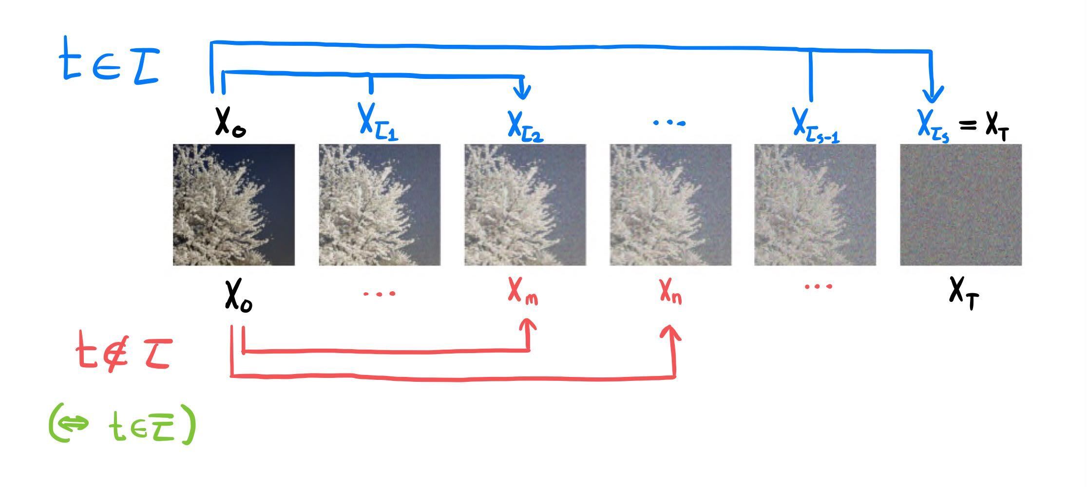
x τ i \mathbf{x}_{\tau_i} x τ i q σ , τ q_{\sigma,\tau} q σ , τ q σ q_\sigma q σ t ∉ τ t \notin \tau t ∈ / τ x t \mathbf{x}_t x t
q σ , τ ( x 1 : T ∣ x 0 ) = q σ , τ ( x τ 1 ∣ x 0 ) ∏ i = 2 S q σ , τ ( x τ i ∣ x τ i − 1 , x 0 ) ∏ t ∉ τ q σ , τ ( x t ∣ x 0 ) q_{\sigma,\tau}(\mathbf{x}_{1:T}~|~\mathbf{x}_0) = q_{\sigma,\tau}(\mathbf{x}_{\tau_1}~|~\mathbf{x}_0)\prod_{i=2}^S q_{\sigma,\tau}(\mathbf{x}_{\tau_i}~|~\mathbf{x}_{\tau_{i-1}},\mathbf{x}_0) \prod_{t\notin\tau} q_{\sigma,\tau}(\mathbf{x}_t~|~\mathbf{x}_0) q σ , τ ( x 1 : T ∣ x 0 ) = q σ , τ ( x τ 1 ∣ x 0 ) i = 2 ∏ S q σ , τ ( x τ i ∣ x τ i − 1 , x 0 ) t ∈ / τ ∏ q σ , τ ( x t ∣ x 0 ) t ∈ τ t \in \tau t ∈ τ ( x τ i − 1 → x τ i ) (\mathbf{x}_{\tau_{i-1}} \to \mathbf{x}_{\tau_i}) ( x τ i − 1 → x τ i ) ( x 0 ) (\mathbf{x}_0) ( x 0 ) t ∉ τ t \notin \tau t ∈ / τ ( x 0 ) (\mathbf{x}_0) ( x 0 )
또한 Bayes Theorem에 의해,
q σ , τ ( x 1 : T ∣ x 0 ) = q σ , τ ( x τ 1 ∣ x 0 ) ∏ i = 2 S q σ , τ ( x τ i ∣ x τ i − 1 , x 0 ) ∏ t ∉ τ q σ , τ ( x t ∣ x 0 ) = q σ , τ ( x τ 1 ∣ x 0 ) ∏ i = 2 S q σ , τ ( x τ i − 1 ∣ x τ i , x 0 ) q σ , τ ( x τ i ∣ x 0 ) q σ , τ ( x τ i − 1 ∣ x 0 ) ∏ t ∉ τ q σ , τ ( x t ∣ x 0 ) = q σ , τ ( x τ S ∣ x 0 ) ∏ i = 2 S q σ , τ ( x τ i − 1 ∣ x τ i , x 0 ) ∏ t ∉ τ q σ , τ ( x t ∣ x 0 ) \begin{aligned} q_{\sigma,\tau}(\mathbf{x}_{1:T}~|~\mathbf{x}_0) &= q_{\sigma,\tau}(\mathbf{x}_{\tau_1}~|~\mathbf{x}_0)\prod_{i=2}^S q_{\sigma,\tau}(\mathbf{x}_{\tau_i}~|~\mathbf{x}_{\tau_{i-1}},\mathbf{x}_0) \prod_{t\notin\tau} q_{\sigma,\tau}(\mathbf{x}_t~|~\mathbf{x}_0) \\ &= q_{\sigma,\tau}(\mathbf{x}_{\tau_1}~|~\mathbf{x}_0)\prod_{i=2}^S {q_{\sigma,\tau}(\mathbf{x}_{\tau_{i-1}}~|~\mathbf{x}_{\tau_i},\mathbf{x}_0)~q_{\sigma,\tau}(\mathbf{x}_{\tau_i}~|~\mathbf{x}_0) \over q_{\sigma,\tau}(\mathbf{x}_{\tau_{i-1}}~|~\mathbf{x}_0)} \prod_{t\notin\tau} q_{\sigma,\tau}(\mathbf{x}_t~|~\mathbf{x}_0) \\ &= q_{\sigma,\tau}(\mathbf{x}_{\tau_S}~|~\mathbf{x}_0)\prod_{i=2}^S q_{\sigma,\tau}(\mathbf{x}_{\tau_{i-1}}~|~\mathbf{x}_{\tau_i},\mathbf{x}_0) \prod_{t\notin\tau} q_{\sigma,\tau}(\mathbf{x}_t~|~\mathbf{x}_0) \\ \end{aligned} q σ , τ ( x 1 : T ∣ x 0 ) = q σ , τ ( x τ 1 ∣ x 0 ) i = 2 ∏ S q σ , τ ( x τ i ∣ x τ i − 1 , x 0 ) t ∈ / τ ∏ q σ , τ ( x t ∣ x 0 ) = q σ , τ ( x τ 1 ∣ x 0 ) i = 2 ∏ S q σ , τ ( x τ i − 1 ∣ x 0 ) q σ , τ ( x τ i − 1 ∣ x τ i , x 0 ) q σ , τ ( x τ i ∣ x 0 ) t ∈ / τ ∏ q σ , τ ( x t ∣ x 0 ) = q σ , τ ( x τ S ∣ x 0 ) i = 2 ∏ S q σ , τ ( x τ i − 1 ∣ x τ i , x 0 ) t ∈ / τ ∏ q σ , τ ( x t ∣ x 0 ) 이다. t ∉ τ t \notin \tau t ∈ / τ x t \mathbf{x}_t x t ( = T ) (=T) ( = T ) q σ q_\sigma q σ
q σ , τ ( x t ∣ x 0 ) = N ( α ˉ t x 0 , ( 1 − α ˉ t ) I ) f o r t = T , e v e r y t ∉ τ q_{\sigma,\tau}(\mathbf{x}_t~|~\mathbf{x}_0) = N(\sqrt{\bar{\alpha}_t}\mathbf{x}_0,~~(1-\bar{\alpha}_t)I)~~~~for~~t=T,~~every~~t\notin\tau q σ , τ ( x t ∣ x 0 ) = N ( α ˉ t x 0 , ( 1 − α ˉ t ) I ) f o r t = T , e v e r y t ∈ / τ 모든 τ i ∈ τ \tau_i \in \tau τ i ∈ τ
q σ , τ ( x τ i − 1 ∣ x τ i , x 0 ) = N ( α ˉ τ i − 1 x 0 + 1 − α ˉ τ i − 1 − σ τ i 2 ⋅ x τ i − α ˉ τ i x 0 1 − α ˉ τ i , σ τ i 2 I ) q_{\sigma,\tau}(\mathbf{x}_{\tau_{i-1}}~|~\mathbf{x}_{\tau_i},\mathbf{x}_0) = N\bigg(\sqrt{\bar{\alpha}_{\tau_{i-1}}}\mathbf{x}_0+\sqrt{1-\bar{\alpha}_{\tau_{i-1}}-\sigma_{\tau_i}^2} \cdot {\mathbf{x}_{\tau_i}-\sqrt{\bar{\alpha}_{\tau_i}}\mathbf{x}_0 \over \sqrt{1-\bar{\alpha}_{\tau_i}}},~~\sigma_{\tau_i}^2I \bigg) q σ , τ ( x τ i − 1 ∣ x τ i , x 0 ) = N ( α ˉ τ i − 1 x 0 + 1 − α ˉ τ i − 1 − σ τ i 2 ⋅ 1 − α ˉ τ i x τ i − α ˉ τ i x 0 , σ τ i 2 I ) 라 정의하자. 이번에도 역시 Appendix B의 Lemma 1에 의해
q σ , τ ( x τ i ∣ x 0 ) = N ( α ˉ τ i x 0 , ( 1 − α ˉ τ i ) I ) f o r e v e r y τ i ∈ τ q_{\sigma,\tau}(\mathbf{x}_{\tau_i}~|~\mathbf{x}_0) = N(\sqrt{\bar{\alpha}_{\tau_i}}\mathbf{x}_0,~~(1-\bar{\alpha}_{\tau_i})I)~~~~for~~every~~\tau_i \in \tau q σ , τ ( x τ i ∣ x 0 ) = N ( α ˉ τ i x 0 , ( 1 − α ˉ τ i ) I ) f o r e v e r y τ i ∈ τ 가 성립한다. [5] 저자는 위의 정의에서 x τ i \mathbf{x}_{\tau_i} x τ i x 0 \mathbf{x}_0 x 0 x 0 \mathbf{x}_0 x 0 x 0 \mathbf{x}_0 x 0
실제 Sampling 역시 부분수열 τ \tau τ p θ p_\theta p θ
p θ ( x 0 : T ) ≔ p θ ( x T ) ∏ i = 1 S p θ ( τ i ) ( x τ i − 1 ∣ x τ i ) ∏ t ∉ τ p θ ( t ) ( x 0 ∣ x t ) p_\theta(\mathbf{x}_{0:T}) \coloneqq p_\theta(\mathbf{x}_T) \prod_{i=1}^S p_\theta^{(\tau_i)} (\mathbf{x}_{\tau_{i-1}}~|~\mathbf{x}_{\tau_i}) \prod_{t \notin \tau} p_\theta^{(t)}(\mathbf{x}_0~|~\mathbf{x}_t) p θ ( x 0 : T ) : = p θ ( x T ) i = 1 ∏ S p θ ( τ i ) ( x τ i − 1 ∣ x τ i ) t ∈ / τ ∏ p θ ( t ) ( x 0 ∣ x t ) 이때 실질적으로 Sampling에 사용되는 p θ ( τ i ) ( x τ i − 1 ∣ x τ i ) p_\theta^{(\tau_i)} (\mathbf{x}_{\tau_{i-1}}~|~\mathbf{x}_{\tau_i}) p θ ( τ i ) ( x τ i − 1 ∣ x τ i )
p θ ( τ i ) ( x τ i − 1 ∣ x τ i ) = q σ , τ ( x τ i − 1 ∣ x τ i , f θ ( τ i ) ( x τ i ) ) p_\theta^{(\tau_i)} (\mathbf{x}_{\tau_{i-1}}~|~\mathbf{x}_{\tau_i}) = q_{\sigma, \tau} (\mathbf{x}_{\tau_{i-1}}~|~\mathbf{x}_{\tau_i}, f_\theta^{(\tau_i)}(\mathbf{x}_{\tau_i})) p θ ( τ i ) ( x τ i − 1 ∣ x τ i ) = q σ , τ ( x τ i − 1 ∣ x τ i , f θ ( τ i ) ( x τ i ) ) 로 정의하며, 그 외 단계들은 다음과 같이 정의한다.
p θ ( t ) ( x 0 ∣ x t ) = N ( f θ ( t ) ( x t ) , σ t 2 I ) p_\theta^{(t)}(\mathbf{x}_0~|~\mathbf{x}_t) = N(f_\theta^{(t)}(\mathbf{x}_t), \sigma_t^2I) p θ ( t ) ( x 0 ∣ x t ) = N ( f θ ( t ) ( x t ) , σ t 2 I )
4-2. Loss Function
앞선 Loss function에서 했던 바와 같이, 모든 σ , τ \sigma, \tau σ , τ J σ , τ ( ϵ θ ) = L γ + C J_{\sigma, \tau} (\epsilon_\theta) = L_\gamma + C J σ , τ ( ϵ θ ) = L γ + C γ t \gamma_t γ t L γ L_\gamma L γ L γ L_\gamma L γ L 1 L_1 L 1 ϵ \epsilon ϵ
관련된 내용은 논문의 Appendix C.1에 기술되어 있지만 증명은 생략되었고, 수식이 논리적으로 전개되지 않으므로 위 증명은 생략하겠다.
4-3. Sampling
결론은 Loss Function이 달라지더라도 최적해의 위치는 DDPMs의 L 1 L_1 L 1
p θ ( x τ i − 1 ∣ x τ i ) = { N ( f θ ( τ 1 ) ( x τ 1 ) , σ τ 1 2 I ) if i = 1 q σ , τ ( x τ i − 1 ∣ x τ i , f θ ( τ i ) ( x τ i ) ) otherwise p_\theta(\mathbf{x}_{\tau_{i-1}}~|~\mathbf{x}_{\tau_i}) = \begin{cases} N(f_\theta^{(\tau_1)}(\mathbf{x}_{\tau_1}), \sigma_{\tau_1}^2I) &\text{if } i=1 \\ q_{\sigma, \tau}(\mathbf{x}_{\tau_{i-1}}~|~\mathbf{x}_{\tau_i}, f_\theta^{(\tau_i)}(\mathbf{x}_{\tau_i})) &\text{otherwise} \end{cases} p θ ( x τ i − 1 ∣ x τ i ) = { N ( f θ ( τ 1 ) ( x τ 1 ) , σ τ 1 2 I ) q σ , τ ( x τ i − 1 ∣ x τ i , f θ ( τ i ) ( x τ i ) ) if i = 1 otherwise 를 이용하여,
x τ i − 1 = { x τ 1 − 1 − α ˉ τ 1 ϵ θ ( τ 1 ) ( x τ 1 ) α ˉ τ 1 + σ τ 1 ϵ τ 1 if i = 1 α ˉ τ i − 1 ⋅ x τ i − 1 − α ˉ τ i ϵ θ ( τ i ) ( x τ i ) α ˉ τ i + 1 − α ˉ τ i − 1 − σ τ i 2 ⋅ ϵ θ ( τ i ) ( x τ i ) + σ τ i ϵ τ i otherwise \mathbf{x}_{\tau_{i-1}} = \begin{cases} {\mathbf{x}_{\tau_1} - \sqrt{1-\bar{\alpha}_{\tau_1}}\epsilon_\theta^{(\tau_1)}(\mathbf{x}_{\tau_1}) \over \sqrt{\bar{\alpha}_{\tau_1}}} +\sigma_{\tau_1}\epsilon_{\tau_1} &\text{if } i=1 \\ \\ \sqrt{\bar{\alpha}_{\tau_{i-1}}} \cdot {\mathbf{x}_{\tau_i} - \sqrt{1-\bar{\alpha}_{\tau_i}}\epsilon_\theta^{(\tau_i)}(\mathbf{x}_{\tau_i}) \over \sqrt{\bar{\alpha}_{\tau_i}}} + \sqrt{1-\bar{\alpha}_{\tau_{i-1}}-\sigma_{\tau_i}^2} \cdot \epsilon_\theta^{(\tau_i)}(\mathbf{x}_{\tau_i}) + \sigma_{\tau_i}\epsilon_{\tau_i} &\text{otherwise} \end{cases} x τ i − 1 = ⎩ ⎪ ⎪ ⎪ ⎪ ⎪ ⎨ ⎪ ⎪ ⎪ ⎪ ⎪ ⎧ α ˉ τ 1 x τ 1 − 1 − α ˉ τ 1 ϵ θ ( τ 1 ) ( x τ 1 ) + σ τ 1 ϵ τ 1 α ˉ τ i − 1 ⋅ α ˉ τ i x τ i − 1 − α ˉ τ i ϵ θ ( τ i ) ( x τ i ) + 1 − α ˉ τ i − 1 − σ τ i 2 ⋅ ϵ θ ( τ i ) ( x τ i ) + σ τ i ϵ τ i if i = 1 otherwise w h e r e ϵ τ i ∼ N ( 0 , I ) where~~\epsilon_{\tau_i} \sim N(0, I) w h e r e ϵ τ i ∼ N ( 0 , I ) 와 같이 Sampling을 진행할 수 있다. Acceleration 이전과 식은 비슷하지만, 부분수열 τ \tau τ 는 점이 큰 차이다.
5. Experiment
σ \sigma σ τ \tau τ σ \sigma σ τ \tau τ
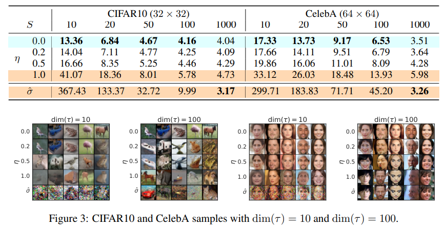
S S S τ \tau τ η \eta η
σ τ i = η ⋅ β t ( 1 − α ˉ t − 1 ) 1 − α ˉ t \sigma_{\tau_i} = \eta \cdot {\beta_t (1-\bar{\alpha}_{t-1}) \over 1-\bar{\alpha}_t} σ τ i = η ⋅ 1 − α ˉ t β t ( 1 − α ˉ t − 1 ) η = 1 \eta = 1 η = 1 σ τ i \sigma_{\tau_i} σ τ i η = 0 \eta = 0 η = 0 η = 1 \eta = 1 η = 1 S = 1000 S=1000 S = 1 0 0 0
평가지표는 FID이며, 값이 작을수록 높은 성능을 의미한다. 전체적으로 S S S η \eta η η = 0 \eta=0 η = 0 σ τ i = 0 \sigma_{\tau_i}=0 σ τ i = 0 S = 1000 S=1000 S = 1 0 0 0 어느정도 성능 하락을 감수하면서 속도를 10배 이상( S ≤ 100 ) (S \le100) ( S ≤ 1 0 0 ) [6]
6. Endnotes
[1] DDPMs의 네트워크는 x t \mathbf{x}_t x t ϵ θ ( t ) \epsilon_\theta^{(t)} ϵ θ ( t ) ( = ϵ θ ( t ) ) (=\epsilon_\theta^{(t)}) ( = ϵ θ ( t ) ) ( = α ˉ t x 0 + 1 − α ˉ t ϵ θ ( t ) = x t ) (= \sqrt{\bar{\alpha}_t}\mathbf{x}_0 + \sqrt{1-\bar{\alpha}_t}\epsilon_\theta^{(t)}=\mathbf{x}_t) ( = α ˉ t x 0 + 1 − α ˉ t ϵ θ ( t ) = x t ) ( = ϵ θ ( t ) ) (=\epsilon_\theta^{(t)}) ( = ϵ θ ( t ) ) x t \mathbf{x}_t x t
q ( x t ∣ x 0 ) = N ( x t ; α ˉ t x 0 , ( 1 − α ˉ t ) I ) q(\mathbf{x}_t~|~\mathbf{x}_0) = N(\mathbf{x}_t~;~\sqrt{\bar{\alpha}_t}\mathbf{x}_0 , (1-\bar{\alpha}_t)I) q ( x t ∣ x 0 ) = N ( x t ; α ˉ t x 0 , ( 1 − α ˉ t ) I ) 인 marginal distribution 뿐이다. 따라서 marginal distribution만 같다면, joint distribution은 무엇이든 상관없다는 아이디어다.
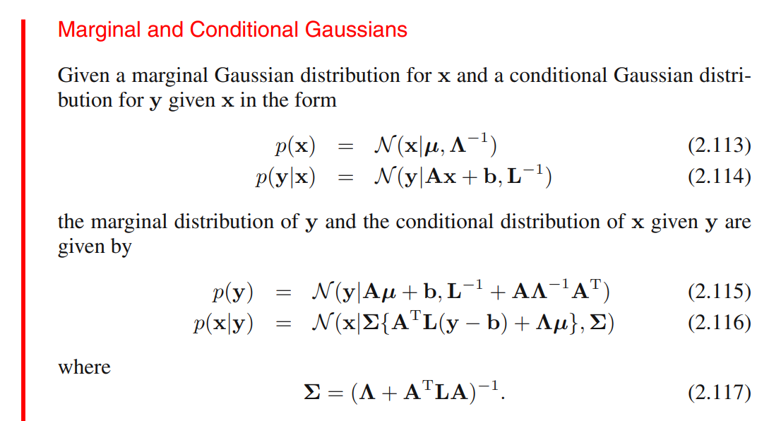
[2] Appendix B의 Lemma 1을 증명하자. 논문은 참고문헌으로 Christopher M Bishop 의 Pattern recognition and machine learning을 인용하였다. 해당 서적에서 참고한 수식은 다음과 같다.
Lemma 1의 증명 아이디어는 수학적 귀납법(Induction)과 유사하다. 다음 두 식
q σ ( x T ∣ x 0 ) = N ( α ˉ T x 0 , ( 1 − α ˉ T ) I ) q_\sigma(\mathbf{x}_T~|~\mathbf{x}_0) = N(\sqrt{\bar{\alpha}_T}\mathbf{x}_0, (1-\bar{\alpha}_T)I) q σ ( x T ∣ x 0 ) = N ( α ˉ T x 0 , ( 1 − α ˉ T ) I ) q σ ( x t − 1 ∣ x t , x 0 ) = N ( α ˉ t − 1 x 0 + 1 − α ˉ t − 1 − σ t 2 ⋅ x t − α ˉ t x 0 1 − α ˉ t , σ t 2 I ) q_\sigma(\mathbf{x}_{t-1}~|~\mathbf{x}_t, \mathbf{x}_0) = N \bigg(\sqrt{\bar{\alpha}_{t-1}}\mathbf{x}_0 + \sqrt{1-\bar{\alpha}_{t-1}-\sigma_t^2} \cdot {\mathbf{x}_t - \sqrt{\bar{\alpha}_t}\mathbf{x}_0 \over \sqrt{1-\bar{\alpha}_t}}, \sigma_t^2I \bigg) q σ ( x t − 1 ∣ x t , x 0 ) = N ( α ˉ t − 1 x 0 + 1 − α ˉ t − 1 − σ t 2 ⋅ 1 − α ˉ t x t − α ˉ t x 0 , σ t 2 I ) 이 정의되었을 때, 모든 t ≤ T t \le T t ≤ T
q σ ( x t ∣ x 0 ) = N ( α ˉ t x 0 , ( 1 − α ˉ t ) I ) ⇓ q σ ( x t − 1 ∣ x 0 ) = N ( α ˉ t − 1 x 0 , ( 1 − α ˉ t − 1 ) I ) q_\sigma(\mathbf{x}_t~|~\mathbf{x}_0) = N(\sqrt{\bar{\alpha}_t}\mathbf{x}_0, (1-\bar{\alpha}_t)I)\\ \Downarrow \\ q_\sigma(\mathbf{x}_{t-1}~|~\mathbf{x}_0) = N(\sqrt{\bar{\alpha}_{t-1}}\mathbf{x}_0, (1-\bar{\alpha}_{t-1})I) q σ ( x t ∣ x 0 ) = N ( α ˉ t x 0 , ( 1 − α ˉ t ) I ) ⇓ q σ ( x t − 1 ∣ x 0 ) = N ( α ˉ t − 1 x 0 , ( 1 − α ˉ t − 1 ) I ) 임을 증명하자. a ⇒ b a \Rightarrow b a ⇒ b a a a b b b
만약 증명된다면, 우리는 이미 t = T t=T t = T q σ ( x T ∣ x 0 ) = N ( α ˉ T x 0 , ( 1 − α ˉ T ) I ) q_\sigma(\mathbf{x}_T~|~\mathbf{x}_0) = N(\sqrt{\bar{\alpha}_T}\mathbf{x}_0, (1-\bar{\alpha}_T)I) q σ ( x T ∣ x 0 ) = N ( α ˉ T x 0 , ( 1 − α ˉ T ) I ) t = T − 1 , ⋯ , 2 , 1 t=T-1,~\cdots,~2,~1 t = T − 1 , ⋯ , 2 , 1
q σ ( x t ∣ x 0 ) = N ( α ˉ t x 0 , ( 1 − α ˉ t ) I ) q_\sigma(\mathbf{x}_t~|~\mathbf{x}_0) = N(\sqrt{\bar{\alpha}_t}\mathbf{x}_0, (1-\bar{\alpha}_t)I) q σ ( x t ∣ x 0 ) = N ( α ˉ t x 0 , ( 1 − α ˉ t ) I ) 가 참이라 가정하자. 만약 x 0 \mathbf{x}_0 x 0
q σ ( x t ) = N ( α ˉ t x 0 , ( 1 − α ˉ t ) I ) q_\sigma(\mathbf{x}_t) = N(\sqrt{\bar{\alpha}_t}\mathbf{x}_0, (1-\bar{\alpha}_t)I) q σ ( x t ) = N ( α ˉ t x 0 , ( 1 − α ˉ t ) I ) 마찬가지로
q σ ( x t − 1 ∣ x t ) = N ( α ˉ t − 1 x 0 + 1 − α ˉ t − 1 − σ t 2 ⋅ x t − α ˉ t x 0 1 − α ˉ t , σ t 2 I ) q_\sigma(\mathbf{x}_{t-1}~|~\mathbf{x}_t) = N \bigg(\sqrt{\bar{\alpha}_{t-1}}\mathbf{x}_0 + \sqrt{1-\bar{\alpha}_{t-1}-\sigma_t^2} \cdot {\mathbf{x}_t - \sqrt{\bar{\alpha}_t}\mathbf{x}_0 \over \sqrt{1-\bar{\alpha}_t}}, \sigma_t^2I \bigg) q σ ( x t − 1 ∣ x t ) = N ( α ˉ t − 1 x 0 + 1 − α ˉ t − 1 − σ t 2 ⋅ 1 − α ˉ t x t − α ˉ t x 0 , σ t 2 I ) 라 표현할 수 있으며, 수식 (2.115)에 의해
q σ ( x t − 1 ) = q σ ( x t − 1 ∣ x 0 ) = N ( α ˉ t − 1 x 0 , ( σ t 2 I + 1 − α ˉ t − 1 − σ t 2 1 − α ˉ t ⋅ ( 1 − α ˉ t ) ) I ) = N ( α ˉ t − 1 x 0 , ( 1 − α ˉ t − 1 ) I ) \begin{aligned} q_\sigma(\mathbf{x}_{t-1}) &= q_\sigma(\mathbf{x}_{t-1}~|~\mathbf{x}_0) \\ &=N \bigg( \sqrt{\bar{\alpha}_{t-1}}\mathbf{x}_0, \bigg( \sigma_t^2I + {1-\bar{\alpha}_{t-1}-\sigma_t^2 \over 1-\bar{\alpha}_t} \cdot (1-\bar{\alpha}_t) \bigg)I \bigg) \\ &= N(\sqrt{\bar{\alpha}_{t-1}}\mathbf{x}_0, (1-\bar{\alpha}_{t-1})I) \end{aligned} q σ ( x t − 1 ) = q σ ( x t − 1 ∣ x 0 ) = N ( α ˉ t − 1 x 0 , ( σ t 2 I + 1 − α ˉ t 1 − α ˉ t − 1 − σ t 2 ⋅ ( 1 − α ˉ t ) ) I ) = N ( α ˉ t − 1 x 0 , ( 1 − α ˉ t − 1 ) I ) 이다. 따라서 수학적 귀납법에 의해, 모든 t ≤ T t \le T t ≤ T
q σ ( x t ∣ x 0 ) = N ( α ˉ t x 0 , ( 1 − α ˉ t ) I ) q_\sigma(\mathbf{x}_t~|~\mathbf{x}_0) = N(\sqrt{\bar{\alpha}_t}\mathbf{x}_0, (1-\bar{\alpha}_t)I) q σ ( x t ∣ x 0 ) = N ( α ˉ t x 0 , ( 1 − α ˉ t ) I ) 가 성립한다.
[3] q σ ( x t − 1 ∣ x t q_\sigma(\mathbf{x}_{t-1}~|~\mathbf{x}_t q σ ( x t − 1 ∣ x t x 0 ) , q σ ( x t ∣ x 0 ) \mathbf{x}_0), q_\sigma(\mathbf{x}_t~|~\mathbf{x}_0) x 0 ) , q σ ( x t ∣ x 0 ) q σ ( x t ∣ x t − 1 , x 0 ) q_\sigma(\mathbf{x}_t~|~\mathbf{x}_{t-1},\mathbf{x}_0) q σ ( x t ∣ x t − 1 , x 0 )
q σ ( x t ∣ x t − 1 , x 0 ) = q σ ( x t − 1 ∣ x t , x 0 ) q σ ( x t ∣ x 0 ) q σ ( x t − 1 ∣ x 0 ) = N ( x t ; μ ~ , Σ ~ ) w h e r e q_\sigma(\mathbf{x}_t~|~\mathbf{x}_{t-1},\mathbf{x}_0) = {q_\sigma(\mathbf{x}_{t-1}~|~\mathbf{x}_t, \mathbf{x}_0)~q_\sigma(\mathbf{x}_t~|~\mathbf{x}_0) \over q_\sigma(\mathbf{x}_{t-1}~|~\mathbf{x}_0)} = N(\mathbf{x}_t~;~\tilde{\mu}, \tilde{\Sigma}) \\ \space\\ where q σ ( x t ∣ x t − 1 , x 0 ) = q σ ( x t − 1 ∣ x 0 ) q σ ( x t − 1 ∣ x t , x 0 ) q σ ( x t ∣ x 0 ) = N ( x t ; μ ~ , Σ ~ ) w h e r e μ ~ = 1 − α ˉ t 1 − α ˉ t − 1 − σ t 2 1 − α ˉ t − 1 x t − 1 + ( α ˉ t − 1 − α ˉ t 1 − α ˉ t − 1 − σ t 2 α ˉ t − 1 1 − α ˉ t − 1 ) x 0 , Σ ~ = σ t 2 ( 1 − α ˉ t ) 1 − α ˉ t − 1 I \tilde{\mu} = {\sqrt{1-\bar{\alpha}_t}\sqrt{1-\bar{\alpha}_{t-1}-\sigma_t^2} \over 1-\bar{\alpha}_{t-1}}\mathbf{x}_{t-1} + \bigg(\sqrt{\bar{\alpha}_t} - {\sqrt{1-\bar{\alpha}_t}\sqrt{1-\bar{\alpha}_{t-1}-\sigma_t^2}\sqrt{\bar{\alpha}_{t-1}} \over 1-\bar{\alpha}_{t-1}}\bigg) \mathbf{x}_0, \\ \space\\ \tilde{\Sigma} = {\sigma_t^2(1-\bar{\alpha}_t) \over 1-\bar{\alpha}_{t-1}}I \kern{275pt} μ ~ = 1 − α ˉ t − 1 1 − α ˉ t 1 − α ˉ t − 1 − σ t 2 x t − 1 + ( α ˉ t − 1 − α ˉ t − 1 1 − α ˉ t 1 − α ˉ t − 1 − σ t 2 α ˉ t − 1 ) x 0 , Σ ~ = 1 − α ˉ t − 1 σ t 2 ( 1 − α ˉ t ) I 으로, Multivariate Gaussian Distribution이다.
사실 q σ ( x t − 1 , x 0 ) q_\sigma(\mathbf{x}_{t-1}, \mathbf{x}_0) q σ ( x t − 1 , x 0 ) x 0 \mathbf{x}_0 x 0 x t − 1 \mathbf{x}_{t-1} x t − 1 q σ ( x t ∣ x t − 1 , x 0 ) q_\sigma(\mathbf{x}_t~|~\mathbf{x}_{t-1},\mathbf{x}_0) q σ ( x t ∣ x t − 1 , x 0 )
[4] 논문에서는 Appendix B의 Theorm 1에 기술되어 있다.
[5] [2] 와 같은 과정이다. t t t τ i \tau_i τ i t − 1 t-1 t − 1 τ i − 1 \tau_{i-1} τ i − 1
[6] η = 0 \eta=0 η = 0 σ τ i = 0 \sigma_{\tau_i}=0 σ τ i = 0
결과론적인 이야기지만 위 상황에 의미를 부여하면, 기존 DDPMs에서 denoising process는 μ θ \mu_\theta μ θ Σ θ \Sigma_\theta Σ θ σ τ i = 0 \sigma_{\tau_i}=0 σ τ i = 0