★[학습목표]
Rankine Cycle Efficiency 와 Heat rate[kJ/kWh]를 계산하는 code를 이해할 수 있다.
Ref) https://github.com/Richard66NZ/steam-cycles-non-ideal/blob/main/04_rankine_reheat_cycle-non-ideal.py
!pip install pyXSteam # python Steam table을 설치
import matplotlib.pyplot as plt # matplotlib를 호출
import numpy as np # numpy 호출
from pyXSteam.XSteam import XSteam
steamTable = XSteam(XSteam.UNIT_SYSTEM_MKS)
print('Rankine reheat cycle analysis (non ideal)')
p1 = 0.06 # State 1 의 압력값을 기준으로 steam table에서
s1 = steamTable.sL_p(p1) # Entropy 값을 찾고
T1 = steamTable.t_ps(p1, s1) # Temperature 값을 찾고
h1 = steamTable.hL_p(p1) # Enthalpy 값을 찾는다.
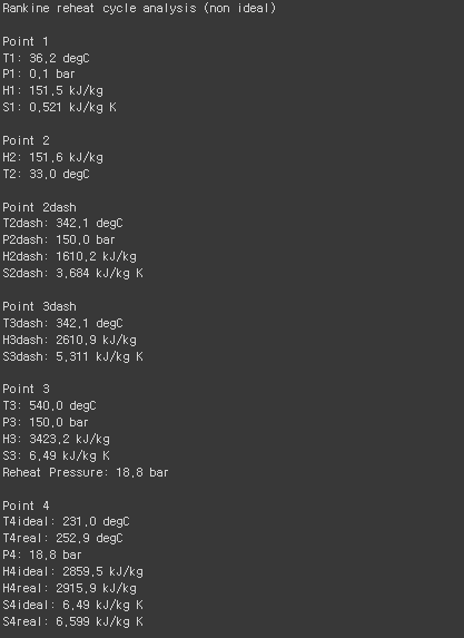
print('\nPoint 1')
print(f"T1: {round(float(T1),1)} degC")
print(f"P1: {round(float(p1),1)} bar")
print(f"H1: {round(float(h1),1)} kJ/kg")
print(f"S1: {round(float(s1),3)} kJ/kg K")
p2 = 150 # 펌프 후단 압력을 150bar로 주어진 값
s2 = s1 # 등엔트로피 조건으로 펌프 작동
v = 1/steamTable.rhoL_p(p1)
w_p = v*(p2-p1)
print('\nPoint 2')
h2 = h1+w_p # State 2에서의 Enthalpy는 h1+펌프동력
print(f"H2: {round(float(h2),1)} kJ/kg")
T2 = steamTable.t_ph(p2, h2) # State 2에서의 P,H 값을 기준으로 T 확인
print(f"T2: {round(float(T2),1)} degC")
h2dash = steamTable.hL_p(p2)
s2dash = steamTable.sL_p(p2)
T2dash = steamTable.t_ph(p2, h2dash)
print('\nPoint 2dash')
print(f"T2dash: {round(float(T2dash),1)} degC")
print(f"P2dash: {round(float(p2),1)} bar")
print(f"H2dash: {round(float(h2dash),1)} kJ/kg")
print(f"S2dash: {round(float(s2dash),3)} kJ/kg K")
h3dash = steamTable.hV_p(p2)
s3dash = steamTable.sV_p(p2)
T3dash = T2dash
print('\nPoint 3dash')
print(f"T3dash: {round(float(T3dash),1)} degC")
print(f"H3dash: {round(float(h3dash),1)} kJ/kg")
print(f"S3dash: {round(float(s3dash),3)} kJ/kg K")
p3 = p2
T3 = 540
h3 = steamTable.h_pt(p3, T3)
s3 = steamTable.s_pt(p3, T3)
print('\nPoint 3')
print(f"T3: {round(float(T3),1)} degC")
print(f"P3: {round(float(p3),1)} bar")
print(f"H3: {round(float(h3),1)} kJ/kg")
print(f"S3: {round(float(s3),3)} kJ/kg K")
p4 = p2/8
print(f"Reheat Pressure: {round(float(p4),1)} bar")
s4 = s3
T4 = steamTable.t_ps(p4, s4)
h4 = steamTable.h_pt(p4, T4)
HPturbeff = 0.90 # HP turbine isentropic efficiency can be entered here (typically 0.85 - 0.95)
h4r = h3 - (HPturbeff * h3) + (HPturbeff * h4)
s4r = steamTable.s_ph(p4, h4r)
T4r = steamTable.t_ps(p4, s4r)
print('\nPoint 4')
print(f"T4ideal: {round(float(T4),1)} degC")
print(f"T4real: {round(float(T4r),1)} degC")
print(f"P4: {round(float(p4),1)} bar")
print(f"H4ideal: {round(float(h4),1)} kJ/kg")
print(f"H4real: {round(float(h4r),1)} kJ/kg")
print(f"S4ideal: {round(float(s4),3)} kJ/kg K")
print(f"S4real: {round(float(s4r ),3)} kJ/kg K")
w_HPt = h3-h4r
p5 = p4
T5 = T3
h5 = steamTable.h_pt(p5, T5)
s5 = steamTable.s_pt(p5, T5)
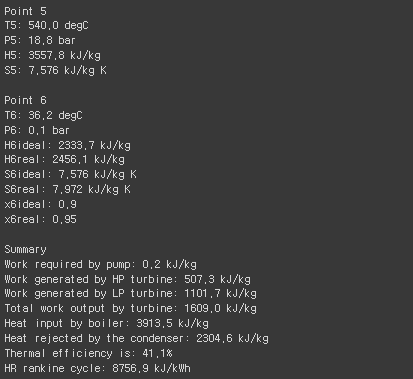
print('\nPoint 5')
print(f"T5: {round(float(T5),1)} degC")
print(f"P5: {round(float(p5),1)} bar")
print(f"H5: {round(float(h5),1)} kJ/kg")
print(f"S5: {round(float(s5),3)} kJ/kg K")
p6 = p1
s6 = s5
T6 = steamTable.t_ps(p6, s6)
x6 = steamTable.x_ps(p6, s6)
h6 = steamTable.h_px(p6, x6)
print('\nPoint 6')
print(f"T6: {round(float(T6),1)} degC")
print(f"P6: {round(float(p6),1)} bar")
LPturbeff = 0.90 # IP/LP turbine isentropic efficiency can be entered here (typically 0.85 - 0.95)
h6r = h5 - (LPturbeff * h5) + (LPturbeff * h6)
print(f"H6ideal: {round(float(h6),1)} kJ/kg")
print(f"H6real: {round(float(h6r),1)} kJ/kg")
s6r = steamTable.s_ph(p6, h6r)
x6r = steamTable.x_ps(p6, s6r)
print(f"S6ideal: {round(float(s6),3)} kJ/kg K")
print(f"S6real: {round(float(s6r ),3)} kJ/kg K")
print(f"x6ideal: {round(float(x6),2)} ")
print(f"x6real: {round(float(x6r),2)} ")
print('\nSummary')
print(f"Work required by pump: {round(float(w_p),1)} kJ/kg")
print(f"Work generated by HP turbine: {round(float(w_HPt),1)} kJ/kg")
w_LPt = h5-h6r
print(f"Work generated by LP turbine: {round(float(w_LPt),1)} kJ/kg")
print(f"Total work output by turbine: {round(float(w_HPt+w_LPt),1)} kJ/kg")
q_H = (h3-h2)+(h5-h4r)
print(f"Heat input by boiler: {round(float(q_H),1)} kJ/kg")
q_L = h6r-h1
print(f"Heat rejected by the condenser: {round(float(q_L),1)} kJ/kg")
eta_th = (w_HPt+w_LPt-w_p)/q_H*100
print(f"Thermal efficiency is: {round(float(eta_th),1)}%")
HRcycle = 3600*100/eta_th
print(f"HR rankine cycle: {round(float(HRcycle),1)} kJ/kWh")
font = {'family' : 'Times New Roman',
'size' : 22}
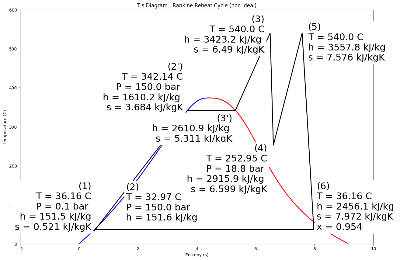
plt.figure(figsize=(15,10))
plt.title('T-s Diagram - Rankine Reheat Cycle (non ideal)')
plt.rc('font', **font)
plt.ylabel('Temperature (C)')
plt.xlabel('Entropy (s)')
plt.xlim(-2,10)
plt.ylim(0,600)
T = np.linspace(0, 373.945, 400) # range of temperatures
# saturated vapor and liquid entropy lines
svap = [s for s in [steamTable.sL_t(t) for t in T]]
sliq = [s for s in [steamTable.sV_t(t) for t in T]]
plt.plot(svap, T, 'b-', linewidth=2.0)
plt.plot(sliq, T, 'r-', linewidth=2.0)
plt.plot([s1, s2, s2dash, s3dash, s3, s4r, s5, s6r, s1],[T1, T2, T2dash, T3dash, T3, T4r, T5, T6, T1], 'black', linewidth=2.0)
plt.text(s1-.1,T1,f'(1)\nT = {round(float(T1),2)} C\nP = {round(float(p1),1)} bar \nh = {round(float(h1),1)} kJ/kg\n s = {round(float(s1),3)} kJ/kgK',
ha='right',backgroundcolor='white')
plt.text(1.6,60,f'(2)\nT = {round(float(T2),2)} C\nP = {round(float(p2),1)} bar \nh = {round(float(h2),1)} kJ/kg',
ha='left',backgroundcolor='white')
plt.text(s2dash-.15,T2dash,f"(2')\nT = {round(float(T2dash),2)} C\nP = {round(float(p2),1)} bar \nh = {round(float(h2dash),1)} kJ/kg \ns = {round(float(s2dash),3)} kJ/kgK",
ha='right',backgroundcolor='white')
plt.text(s3dash-.1,T3dash-80,f"(3')\nh = {round(float(h3dash),1)} kJ/kg \ns = {round(float(s3dash),3)} kJ/kgK",
ha='right',backgroundcolor='white')
plt.text(6.3,T3-50,f'(3)\nT = {round(float(T3),2)} C\nh = {round(float(h3),1)} kJ/kg \ns = {round(float(s3),3)} kJ/kgK',
ha='right',backgroundcolor='white')
plt.text(s4-.1,T4r-120,f'(4)\nT = {round(float(T4r),2)} C\nP = {round(float(p4),1)} bar \nh = {round(float(h4r),1)} kJ/kg \ns = {round(float(s4r),3)} kJ/kgK',
ha='right',backgroundcolor='white')
plt.text(s5+.2,T5-70,f'(5)\nT = {round(float(T5),2)} C\nh = {round(float(h5),1)} kJ/kg \ns = {round(float(s5),3)} kJ/kgK',
ha='left',backgroundcolor='white')
plt.text(s6r+.1,T6,f'(6)\nT = {round(float(T6),2)} C\nh = {round(float(h6r),1)} kJ/kg \ns = {round(float(s6r),3)} kJ/kgK \nx = {round(float(x6r),3)}',
ha='left',backgroundcolor='white')
plt.savefig('04-rankine-reheat-cycle-non-ideal-TSdiagram.png')