
1. Linear Regression 실습
: 자동차 연비 예측
차량의 연비를 예측하는 모델을 만드려고 함
자동차의 특성을 기반으로 연비를 예측하는 선형회귀 모델을 학습
Step1. 데이터 생성하기
import numpy as np
import matplotlib.pyplot as plt

# 데이터 생성하기

np.random.seed(42)
cc=np.random.randint(1000,3500,size=50)
epsilon=np.random.normal(0,1,size=50)

#파라메터 w,b 초기화
w=0.0037
b=0.0
l=w*cc+b+epsilon

plt.scatter(cc,l)
plt.xlabel('cc')
plt.ylabel('l')
plt.show()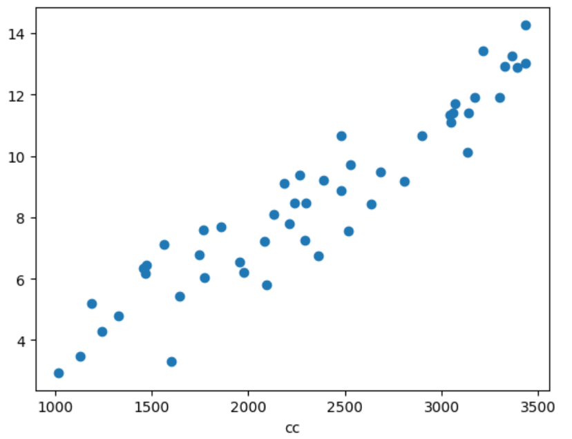
Step2. Model 만들기 (클래스 형태로 모델 생성)
2.1) 초기화 함수 정의하기 : w,b 랜덤함수 사용하여 0.0~1.0 값으로 정의
2.2) 모델을 정의 : prediction 함수를 만들고, 입력 들어오면 예측 결과 출력
2.3) 출력 시각화 : 모델 초기화, 1.1에서 만든 배기량을 입력했을 때, 출력을 받아 plot
class LinearRegression :
  def __init__(self, learning_rate=0, n_interations=0):
    self.learning_rate=learning_rate
    self.n_interations=n_interations
    np.random.seed(42)
    self.weights=np.random.randn(1)
    self.bias=np.random.randn(1)

  def predict(self, X):
    return self.weights*X+self.bias

model=LinearRegression()
pred=model.predict(cc)

plt.scatter(cc,l)
plt.plot(cc, pred, color='red')
plt.xlabel('cc')
plt.ylabel('l/kl')
plt.show()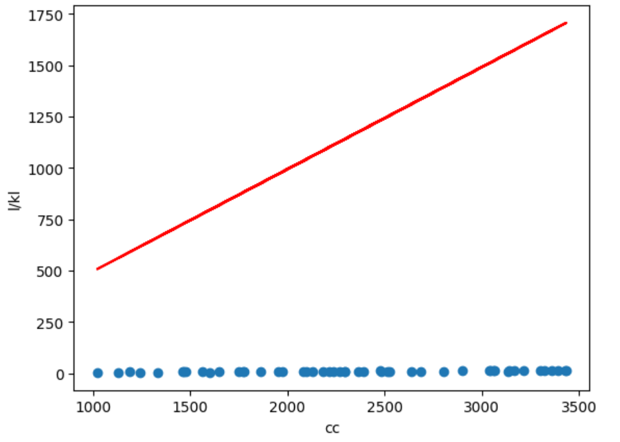
Step3. Model 학습 코드 (fit 함수)
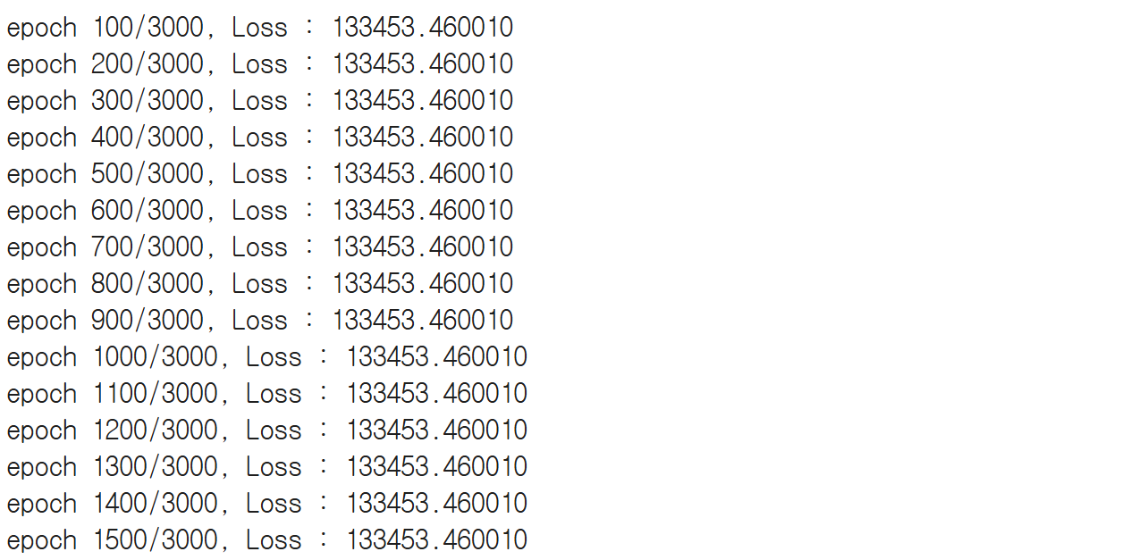
3.1 ) 앞에서 만든 클래스 내부에, 학습을 위한 fit 함수 만들기 : Gradient Descent 구현 후 w,b 학습
(Learning rate : 1e-10, epoch : 3000)
3.2 ) 실시간 학습 결과 출력하기 : 학습 과정 100회 반복마다 학습 횟수와 현재 loss값 출력하도록 수정
class LinearRegression :
  def __init__(self, learning_rate=1e-10, n_interations=1000):
    self.learning_rate=learning_rate
    self.n_interations=n_interations
    np.random.seed(42)
    self.weights=np.random.randn(1)
    self.bias=np.random.randn(1)

  def fit(self, X,y):
    for i in range(self.n_interations):
      y_pred=self.predict(X)

      current_loss=np.mean((y-pred)**2)

      dw=np.mean(2*X*(y_pred-y))
      db=np.mean(2*(y_pred-y))

      self.weights=self.weights-self.learning_rate*dw
      self.bias=self.bias-self.learning_rate*db

      #100회 반복마다 학습 횟수와 loss값 출력
      if (i+1)%100==0:
        print(f'epoch {i+1}/{self.n_interations}, Loss : {current_loss:.6f}')

  def predict(self, X):
    return self.weights*X+self.bias
Step4. 모델 학습하기
4.1 ) 생성한 모델을 활용하여 모델 만들고, fit 함수를 이용하여 학습
model=LinearRegression()
model.fit(cc, l)
pred=model.predict(cc)

plt.scatter(cc,l)
plt.plot(cc, pred, color='red')
plt.xlabel('cc')
plt.ylabel('l/kl')
plt.show()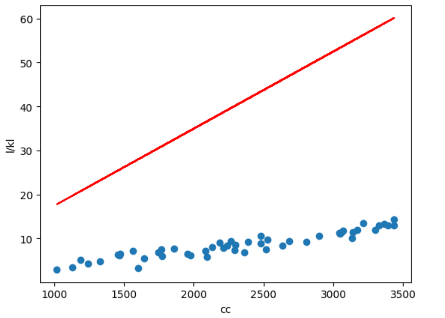
Step5. 하이퍼 파라미터에 따른 학습 결과 관찰
5.1 ) 학습률을 1e-5, 1e-20으로 세팅 후 학습결과 관찰
5.2 ) 학습률을 1e-10, epoch이 3000, 10,000일 때 학습 결과 관찰
Step6. 데이터 정규화
6.1 ) sklearn의 MinMaxScaler를 이용하여 입력 x, 출력 y를 각각 정규화
from sklearn.preprocessing import MinMaxScaler

#MinMax Scaling (0,1사이로 정규화)
scaler_x=MinMaxScaler()
scaler_y=MinMaxScaler()

cc=cc.reshape(-1,1)
l=l.reshape(-1,1)

scaler_x.fit(cc)
scaler_y.fit(l)

X_scaled_minmax=scaler_x.transform(cc)
y_scaled_minmax=scaler_y.transform(l)
6.2 ) 정규화된 데이터 출력
plt.scatter(X_scaled_minmax,y_scaled_minmax)
plt.xlabel('cc')
plt.ylabel('l/kl')
plt.show()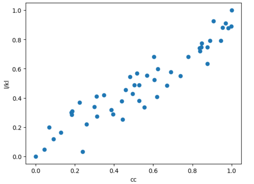
Step7. 데이터 정규화 및 모델 재학습
7.1 ) 하이퍼파라메터를 1e-3으로 epoch 3,000 설정하여 모델을 재학습
class LinearRegression:
    def __init__(self, learning_rate=1e-3, n_interations=3000):
        self.learning_rate = learning_rate
        self.n_interations = n_interations
        np.random.seed(42)
        self.weights = np.random.randn(1)
        self.bias = np.random.randn(1)

    def fit(self, X, y):
        for i in range(self.n_interations):
            y_pred = self.predict(X)
            current_loss = np.mean((y - y_pred)**2)

            dw = np.mean(2 * X * (y_pred - y))
            db = np.mean(2 * (y_pred - y))

            self.weights -= self.learning_rate * dw
            self.bias -= self.learning_rate * db

            if (i + 1) % 100 == 0:
                print(f'Iteration {i + 1}/{self.n_interations}, Loss: {current_loss:.6f}')

    def predict(self, X):
        return self.weights * X + self.bias

# MinMax 정규화
scaler_x = MinMaxScaler()
scaler_y = MinMaxScaler()

cc = cc.reshape(-1, 1)
l = l.reshape(-1, 1)

scaler_x.fit(cc)
scaler_y.fit(l)

X_scaled_minmax = scaler_x.transform(cc)
y_scaled_minmax = scaler_y.transform(l)

# 모델 학습
model1 = LinearRegression(learning_rate=1e-3, n_interations=3000)
model1.fit(X_scaled_minmax, y_scaled_minmax)

# 예측 및 inverse transform
pred_scaled = model1.predict(X_scaled_minmax)
pred_original = scaler_y.inverse_transform(pred_scaled)

# 결과 출력
plt.scatter(cc, l)
plt.plot(cc, pred_original, color='red')
plt.xlabel('cc')
plt.ylabel('l/kl')
plt.title('학습 후')
plt.show()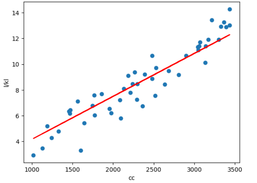
2. Logistic Regression 실습
Step1. 데이터 생성
import numpy as np
import matplotlib.pyplot as plt

#데이터 생성하기
np.random.seed(42)
cc=np.cumsum(np.random.randint(10,150, size=50)) +1000
ton=np.cumsum(np.random.randint(10,200, size=50)) +1000
mph=np.cumsum(np.random.randint(10,50, size=50)) +500

epsilon=np.random.normal(0,1,size=50)

W=[0.0013, 0.004, 0.002]
b=10.0
X=[cc, ton, mph]
l=W[0]*cc + W[1]*ton + W[2]*mph + b +epsilon
Step2. 데이터 시각화
plt.figure(figsize=(15,5))
plt.subplot(1,3,1)
plt.scatter(cc,l)
plt.xlabel('cc')
plt.ylabel('l/km')

plt.subplot(1,3,2)
plt.scatter(ton,l)
plt.xlabel('ton')
plt.ylabel('l/km')

plt.subplot(1,3,3)
plt.scatter(mph,l)
plt.xlabel('mph')
plt.ylabel('l/km')
plt.show()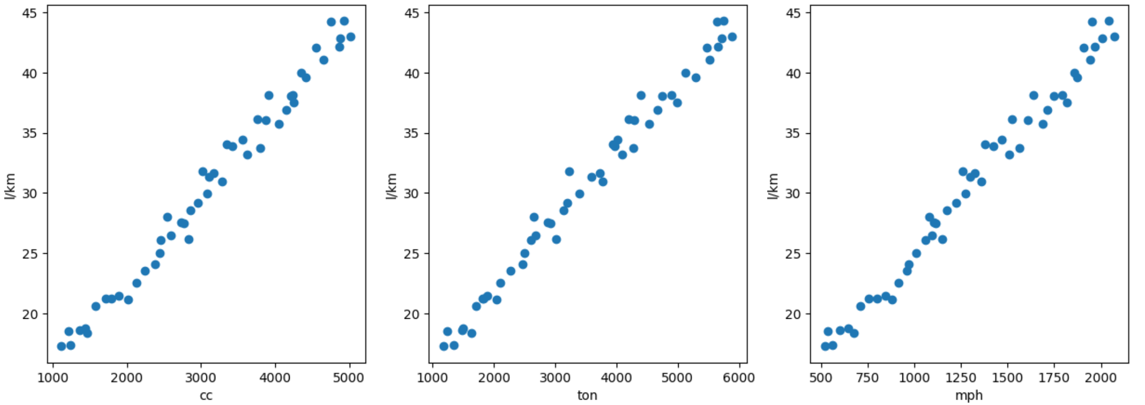
Step3. Model 만들기
3.1 ) 모델 클래스를 만들고 초기화 함수를 작성
3.2 ) Loss 함수 만들기
3.3 ) Predict 함수 만들기
3.4 ) 학습하기 (fit함수 만들기)
class LinearRegression:
  def __init__(self, learning_rate=1e-20, n_iterations=30000):
    self.learning_rate = learning_rate
    self.n_iterations = n_iterations

    np.random.seed(42)
    self.w1 = np.random.uniform(-0.1, 0.1)
    self.w2 = np.random.uniform(-0.1, 0.1)
    self.w3 = np.random.uniform(-0.1, 0.1)
    self.bias = np.random.uniform(-0.1, 0.1)

  def compute_loss(self, y_true, y_pred):
    """MSE Loss 계산"""
    return np.mean((y_true- y_pred) ** 2)

  def fit(self, X, y):
    m = len(X) # 데이터 샘플 수
    for i in range(self.n_iterations):

      y_pred = self.predict(X)   # 예측값 계산
      current_loss = self.compute_loss(y, y_pred) # 현재 loss 계산 및 저장

      # Gradient 계산
      dw1 = (2/m) * np.sum(X[:,0] * (y_pred- y))
      dw2 = (2/m) * np.sum(X[:,1] * (y_pred- y))
      dw3 = (2/m) * np.sum(X[:,2] * (y_pred- y))
      db = (2/m) * np.sum(y_pred- y)

      # 파라미터 업데이트
      self.w1 = self.w1- self.learning_rate * dw1
      self.w2 = self.w2- self.learning_rate * dw2
      self.w3 = self.w3- self.learning_rate * dw3
      self.bias = self.bias- self.learning_rate * db

      # 학습 과정 출력 (100회 반복마다)
      if (i + 1) % 100 == 0:
        print(f'Iteration {i+1}/{self.n_iterations}, Loss: {current_loss:.6f}')

  def predict(self, X):
    return X[:,0] * self.w1 + X[:,1] * self.w2 + X[:,2] * self.w3 + self.bias
Step4. Model 초기화 및 학습
# cc, ton, mph를 세로로 묶어줘야 해요
X = np.column_stack((cc, ton, mph))
l = l.reshape(-1, 1)

# 모델 생성 및 학습
model = LinearRegression()
model.fit(X, l)

# 예측
pred = model.predict(X)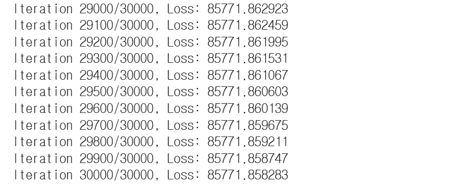
Step5. 결과 시각화
# 시각화
plt.scatter(pred, l, color='red')
plt.xlabel('pred')
plt.ylabel('l/kl')
plt.show()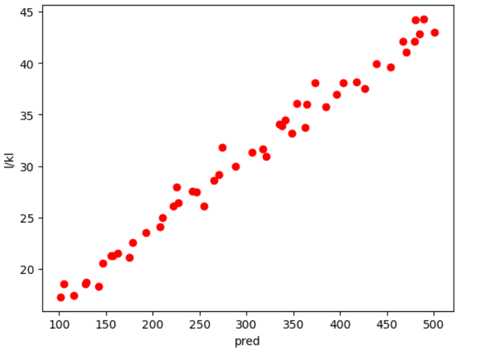
Step6. 데이터 정규화 (Normalization)
from sklearn.preprocessing import MinMaxScaler
# 1. Min-Max Scaling (0~1 사이로 정규화)
minmax_scaler_x1=MinMaxScaler()
minmax_scaler_x2=MinMaxScaler()
minmax_scaler_x3=MinMaxScaler()
minmax_scaler_y=MinMaxScaler()
cc=cc.reshape(-1,1)
ton=ton.reshape(-1,1)
mph=mph.reshape(-1,1)
l=np.array(l).reshape(-1,1)
X_scaled_minmax1=minmax_scaler_x1.fit_transform(cc)
X_scaled_minmax2=minmax_scaler_x2.fit_transform(ton)
X_scaled_minmax3=minmax_scaler_x3.fit_transform(mph)
X_scaled_minmax=np.concatenate([X_scaled_minmax1, X_scaled_minmax2, X_scaled_minmax3], axis=1)
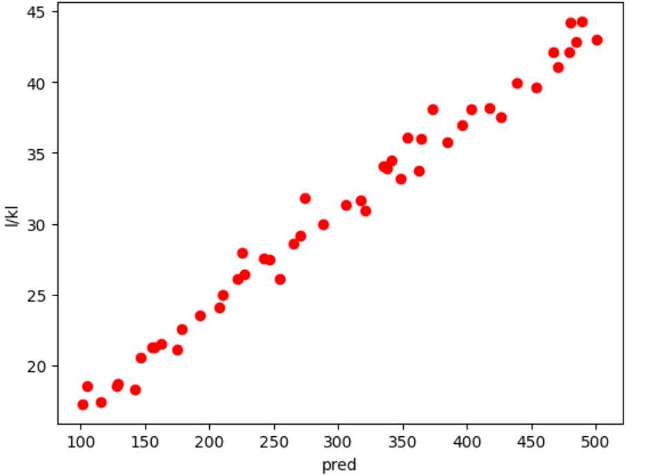
y_scaled_minmax=minmax_scaler_y.fit_transform(l)Step7. 데이터 정규화 및 모델 재학습
# cc, ton, mph를 세로로 묶어줘야 해요
X_scaled_minmax_ = np.column_stack((X_scaled_minmax1, X_scaled_minmax2, X_scaled_minmax3))
l_scaled_minmax_ = l.reshape(-1, 1)

# 모델 생성 및 학습
model1 = LinearRegression()
model1.fit(X_scaled_minmax_, l_scaled_minmax_)

# 예측
pred = model1.predict(X)

# 시각화
plt.scatter(pred, l_scaled_minmax_, color='red')
plt.xlabel('pred')
plt.ylabel('l/kl')
plt.show()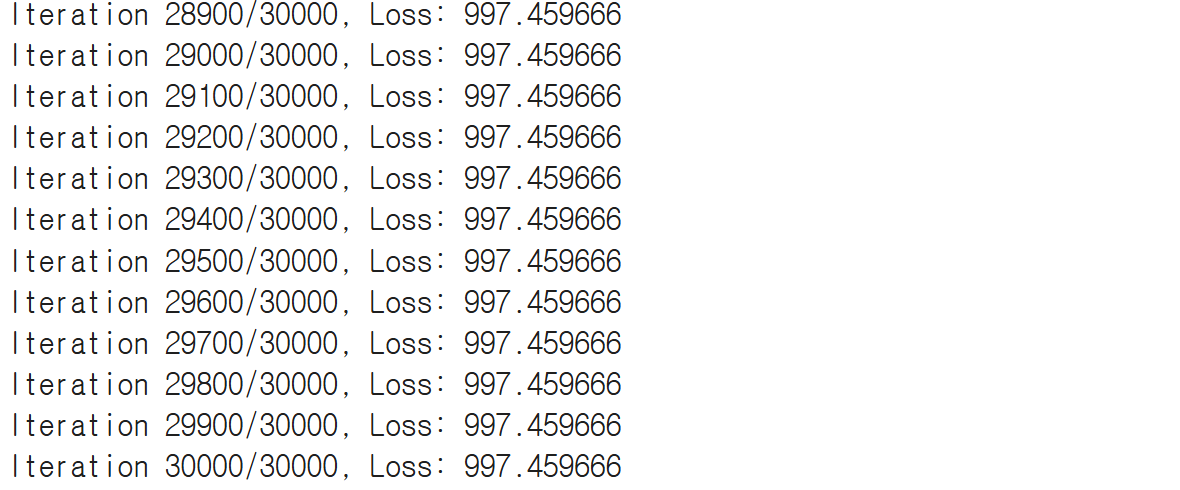

안녕하세요 :)