머신러닝(파이썬) - Sobel Filtering(1)

교육 정보

• 교육 명: 경기미래기술학교 AI 교육
• 교육 기간: 2023.05.08 ~ 2023.10.31
• 오늘의 커리큘럼:
  파이썬 기반의 머신러닝 이해와 실습 (06/14~07/07)
• 강사: 양정은 강사님
• 강의 계획:
  1. 개발환경세팅 - IDE, 가상환경
  2. 인공지능을 위한 Python
  3. KNN 구현을 위한 NumPy
  4. K Nearest Neighbors Classification 구현
  5. K Means Clustering Mini-project
  6. Scikit-learn을 이용한 SVM의 학습
  7. Decision Tree의 개념
  8. ID3 Algorithm
  9. Impurity Metrics - Information Gain Ratio, Gini Index
  10. Decision Tree 구현
  11. 확률 기초
  12. Bayes 정리 예시
  13. Naive Bayes Classifier
  14. Gaussian Naive Bayes Classifier

Sobel Filtering

• 이미지 필터링
• 머신러닝, 딥러닝에서 많이쓰이는 연산
  
  

연습

• 행렬 기본 연산

tmp = np.ones(shape=(2, 3))
print(tmp, '\n')

tmp2 = tmp * 10
print(tmp2)
#
# 결과
[[1. 1. 1.]
 [1. 1. 1.]] 

[[10. 10. 10.]
 [10. 10. 10.]]

이미지 출력

• 흑백 이미지 출력

# 흑백 이미지 만들기
white_patch = 255*np.ones(shape=(10, 10))
black_patch = 0*np.ones(shape=(10, 10))

img3 = np.hstack([white_patch, black_patch, white_patch])
img4 = np.hstack([black_patch, white_patch, black_patch])

img_2 = np.vstack([img3, img4, img3])

• array 반복 (원소별, 전체 패턴)

data = np.arange(5)
print(data)

# np.repeat 원소별 반복
print('repeat:', np.repeat(data, repeats=3))

# np.tile 전체 반복
print('tile:', np.tile(data, reps=3))
#
# 결과
[0 1 2 3 4]
repeat: [0 0 0 1 1 1 2 2 2 3 3 3 4 4 4]
tile: [0 1 2 3 4 0 1 2 3 4 0 1 2 3 4]

• array (axis 지정)

data = np.arange(6).reshape(2, 3)
print(data)

print('repeat(axis=0):', '\n', np.repeat(data, repeats=3, axis=0))
# print(data.repeat(repeats=3, axis=0))
print('repeat(axis=1):', '\n', np.repeat(data, repeats=3, axis=1))
# print(data.repeat(repeats=3, axis=1))
print('repeat(axis=0 & axis=1):', '\n', np.repeat(np.repeat(data, repeats=2, axis=0), repeats=3, axis=1))
# print(data.repeat(repeats=2, axis=0).repeat(repeats=3, axis=1))
#
# 결과
repeat(axis=0): 
 [[0 1 2]
 [0 1 2]
 [0 1 2]
 [3 4 5]
 [3 4 5]
 [3 4 5]]
repeat(axis=1): 
 [[0 0 0 1 1 1 2 2 2]
 [3 3 3 4 4 4 5 5 5]]
repeat(axis=0 & axis=1): 
 [[0 0 0 1 1 1 2 2 2]
 [0 0 0 1 1 1 2 2 2]
 [3 3 3 4 4 4 5 5 5]
 [3 3 3 4 4 4 5 5 5]]

• tile (axis)

data = np.arange(6).reshape(2, 3)
print(data)

print('tile(axis=0):\n',
      np.tile(data, reps=[3, 1]))
print('tile(axis=1):\n',
      np.tile(data, reps=[1, 3]))
print('tile(axis=0 & axis=1):\n',
      np.tile(data, reps=[3, 3]))
#
# 결과
[[0 1 2]
 [3 4 5]]
 
tile(axis=0):
 [[0 1 2]
 [3 4 5]
 [0 1 2]
 [3 4 5]
 [0 1 2]
 [3 4 5]]
 
tile(axis=1):
 [[0 1 2 0 1 2 0 1 2]
 [3 4 5 3 4 5 3 4 5]]
 
tile(axis=0 & axis=1):
 [[0 1 2 0 1 2 0 1 2]
 [3 4 5 3 4 5 3 4 5]
 [0 1 2 0 1 2 0 1 2]
 [3 4 5 3 4 5 3 4 5]
 [0 1 2 0 1 2 0 1 2]
 [3 4 5 3 4 5 3 4 5]]

• 이미지 타일로 만들기 (1)

white_patch = 255*np.ones(shape=(10, 10))
black_patch = 0*np.ones(shape=(10, 10))

img1 = np.hstack([white_patch, black_patch])
img2 = np.hstack([black_patch, white_patch])

img = np.vstack([img1, img2])

img_extend = np.tile(img, reps=[4,4])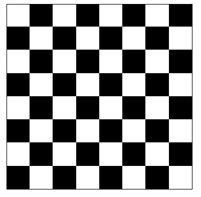

• 이미지 타일로 만들기 (2)

white_patch = 255*np.ones(shape=(10, 10))
gray_patch = 122*np.ones(shape=(10, 10))
black_patch = 0*np.ones(shape=(10, 10))

img1 = np.hstack([white_patch, gray_patch])
img2 = np.hstack([gray_patch, black_patch])

img = np.vstack([img1, img2])

img_extend = np.tile(img, reps=[4, 4])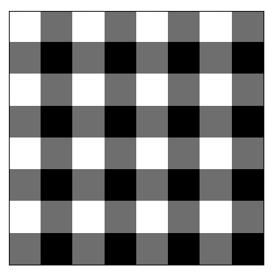

• 이미지 repeat (1)
  - gray scale을 숫자로 지정하고 따로 범위 설정 하지 않으면 최소값을 0 최대값을 255으로 알아서 plot 함

img = np.arange(0, 256, 50).reshape(1,-1)
# img = np.arange(5).reshape(1,-1)

img = img.repeat(repeats=100, axis=0).repeat(repeats=30, axis=1)

fig, ax = plt.subplots()
ax.imshow(img, cmap='gray')

ax.tick_params(left=False, labelleft=False,
               bottom=False, labelbottom=False)
plt.show()

• 이미지 repeat (2, cmap 범위 지정)
  - cmap의 범위를 0-255로 지정했으므로 이미지 array의 최소값인 65가 0(흰색)이 아니라 65(회색)으로 plot됨

img = np.arange(0, 256, 65).reshape(1, -1)
img = img.repeat(repeats=100, axis=0).repeat(repeats=30, axis=1)

fig, ax = plt.subplots()
ax.imshow(img, cmap='gray', vmax=255, vmin=0)
ax.tick_params(left=False, labelleft=False,
               bottom=False, labelbottom=False)
plt.show()

• 이미지 repeat (3)

img = np.arange(5, -1, -1).reshape(-1, 1)
# img = np.arange(5)[::-1].reshape(-1, 1)
img = img.repeat(repeats=30, axis=0).repeat(repeats=100, axis=1)

• 이미지 repeat (4)

img1 = np.arange(0, 256).reshape(1, -1)
img1 = np.repeat(img1, repeats=100, axis=0)
img2 = np.arange(0, 256)[::-1].reshape(1, -1)
img2 = np.repeat(img2, repeats=100, axis=0)

img = np.vstack([img1, img2])

윈도우

• 1-Dimensional Window Extraction
  ✏️ 윈도우의 개수 = 전체 길이 - 윈도우 길이 + 1

data = 10*np.arange(1, 11)
L = len(data)
W = 3
print(data, '\n')

L_ = L - W + 1
for idx in range(L_):
    print(data[idx:idx + W])
#
# 결과
[ 10  20  30  40  50  60  70  80  90 100] 

[10 20 30]
[20 30 40]
[30 40 50]
[40 50 60]
[50 60 70]
[60 70 80]
[70 80 90]
[ 80  90 100]

• 2-Dimensional Window Extraction

• 2차원 배열에서 filter의 갯수
  = 전체 데이터 길이 - 윈도우 길이 + 1
  = (전체 데이터 행의 길이-윈도우 행의 길이+1)
     * (전체 데이터 열의 길이-윈도우 열의 길이+1)

data = 10*np.arange(1, 8).reshape(1, -1)
# data = data.repeat(repeats=5, axis=0)
'''📌 브로드캐스팅 때문에 위 코드가 필요없음!!!'''
adding = 10*np.arange(0, 5).reshape(-1, 1)
data = data + adding

L1 = len(data)
W1 = 3
L1_ = L1-W1+1

L2 = len(data[0])
W2 = 3
L2_ = L2-W2+1

'''📌 위에서 L1, L2는 L1, L2 = data.shape로 받아올수도 있음'''

for r_idx in range(L1_):
    for c_idx in range(L2_):
        print(data[r_idx: r_idx+W1, c_idx:c_idx+W2])
#
# 결과
[[10 20 30]
 [20 30 40]
 [30 40 50]]
[[20 30 40]
 [30 40 50]
 [40 50 60]]
 ...
 [[ 70  80  90]
 [ 80  90 100]
 [ 90 100 110]]

Correlation

data에서 window를 뽑고 filter와 곱한 결과를 저장

• window와 filter가 같을때 가장 큰 값을 출력
• window와 filter가 반대일때 가장 작은 값을 출력

• 1-D Correlation
  - 📌 numpy.dot 사용

import numpy as np

np.random.seed(0)

data = np.random.randint(-1, 2, (10,))
filter_ = np.array([-1, 1, -1])

print(f'{data = }')
print(f'{filter_ = }')

L = len(data)
F = len(filter_)

L_ = L - F + 1
filtered = []

for idx in range(L_):
    window = data[idx:idx + F]
    filtered.append(np.dot(window, filter_))

filtered = np.array(filtered)
print('filtering result:', filtered)
#
# 결과
data = array([-1,  0, -1,  0,  0,  1, -1,  1, -1, -1])
filter_ = array([-1,  1, -1])
filtering result: [ 2 -1  1 -1  2 -3  3 -1]

• 2-D Correlation
  - 📌 numpy.dot을 사용하지 않음! (행렬 내적이 아닌 행렬곱)

import numpy as np
data = 10*np.arange(1, 8).reshape(1, -1)
adding = 10*np.arange(0, 5).reshape(-1, 1)
data = data + adding
print(f'{data = }\n')

ft = np.array([1, 2, 5, -10, 2, -2, 5, 1, -4]).reshape(3, 3)
print(f'{ft = }\n')

H, W = data.shape
F = len(ft)
# print(H, W, F)

H_ = H - F + 1
W_ = W - F + 1

filtered = list()
for h_idx in range(H_):
    for w_idx in range(W_):
        window = data[h_idx:h_idx + F, w_idx:w_idx + F]
        filtered.append((window * ft).sum())

filtered = np.array(filtered).reshape(H_, W_)
print(f'{filtered = }\n')
#
# 결과
data = array([[ 10,  20,  30,  40,  50,  60,  70],
       [ 20,  30,  40,  50,  60,  70,  80],
       [ 30,  40,  50,  60,  70,  80,  90],
       [ 40,  50,  60,  70,  80,  90, 100],
       [ 50,  60,  70,  80,  90, 100, 110]])

ft = array([[  1,   2,   5],
       [-10,   2,  -2],
       [  5,   1,  -4]])

filtered = array([[-30, -30, -30, -30, -30],
       [-30, -30, -30, -30, -30],
       [-30, -30, -30, -30, -30]])