01. Analysis Seoul CCTV
목표
- 서울시 구별 CCTV 현황 데이터 확보
- 서울시 구별 인구 현황 데이터 확보
- CCTV 데이터와 인구 현황 데이터 합치기
- 데이터를 정리하고 정렬하기
- 그래프를 그릴 수 있는 능력
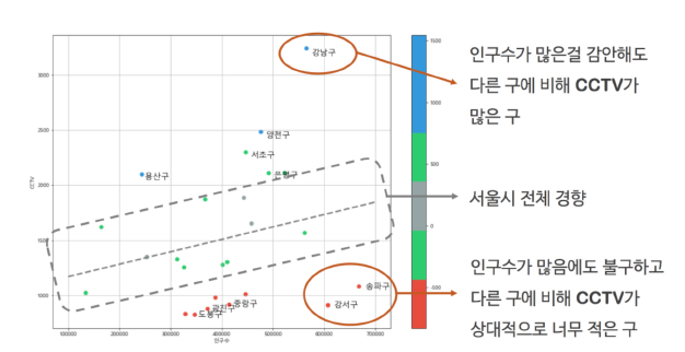
- 전제적인 경향을 파악할 수 있는 능력
- 그 경향에서 벗어난 데이터를 강조하는 능력
1. 데이터 읽기
import pandas as pd
CCTV_Seoul = pd.read_csv("../data/01. Seoul_CCTV.csv")
CCTV_Seoul.head()
|
기관명 |
소계 |
2013년도 이전 |
2014년 |
2015년 |
2016년 |
| 0 |
강남구 |
3238 |
1292 |
430 |
584 |
932 |
| 1 |
강동구 |
1010 |
379 |
99 |
155 |
377 |
| 2 |
강북구 |
831 |
369 |
120 |
138 |
204 |
| 3 |
강서구 |
911 |
388 |
258 |
184 |
81 |
| 4 |
관악구 |
2109 |
846 |
260 |
390 |
613 |
CCTV_Seoul.tail()
|
기관명 |
소계 |
2013년도 이전 |
2014년 |
2015년 |
2016년 |
| 20 |
용산구 |
2096 |
1368 |
218 |
112 |
398 |
| 21 |
은평구 |
2108 |
1138 |
224 |
278 |
468 |
| 22 |
종로구 |
1619 |
464 |
314 |
211 |
630 |
| 23 |
중구 |
1023 |
413 |
190 |
72 |
348 |
| 24 |
중랑구 |
916 |
509 |
121 |
177 |
109 |
CCTV_Seoul.columns
Index(['기관명', '소계', '2013년도 이전', '2014년', '2015년', '2016년'], dtype='object')
CCTV_Seoul.columns[0]
'기관명'
CCTV_Seoul.rename(columns={CCTV_Seoul.columns[0]:"구별"}, inplace=True)
CCTV_Seoul.head()
|
구별 |
소계 |
2013년도 이전 |
2014년 |
2015년 |
2016년 |
| 0 |
강남구 |
3238 |
1292 |
430 |
584 |
932 |
| 1 |
강동구 |
1010 |
379 |
99 |
155 |
377 |
| 2 |
강북구 |
831 |
369 |
120 |
138 |
204 |
| 3 |
강서구 |
911 |
388 |
258 |
184 |
81 |
| 4 |
관악구 |
2109 |
846 |
260 |
390 |
613 |
pop_Seoul = pd.read_excel(
    "../data/01. Seoul_Population.xls", header=2, usecols="B, D, G, J, N "
)
pop_Seoul.head()
|
자치구 |
계 |
계.1 |
계.2 |
65세이상고령자 |
| 0 |
합계 |
10124579 |
9857426 |
267153 |
1365126 |
| 1 |
종로구 |
164257 |
154770 |
9487 |
26182 |
| 2 |
중구 |
134593 |
125709 |
8884 |
21384 |
| 3 |
용산구 |
244444 |
229161 |
15283 |
36882 |
| 4 |
성동구 |
312711 |
304808 |
7903 |
41273 |
pop_Seoul.rename(
    columns={
        pop_Seoul.columns[0]: "구별",
        pop_Seoul.columns[1]: "인구수",
        pop_Seoul.columns[2]: "한국인",
        pop_Seoul.columns[3]: "외국인",
        pop_Seoul.columns[4]: "고령자"
    },
    inplace=True
)
Pandas 기초
- python에서 R만큼의 강력한 데이터 핸들링 성능을 제공하는 모듈
- 단일 프로세스에서는 최대 효율
- 코딩 가능하고 응용 가능한 엑셀로 받아들여도 됨.
Series 데이터 타입
- index와 value로 이루어짐
- 한 가지 데이터 타입만 가질 수 있다.
import pandas as pd
import numpy as np
- pandas는 통상 pd
- numpy는 통상 np 로 설정
pd.Series([1,2,3,4])
0    1
1    2
2    3
3    4
dtype: int64
pd.Series([1,2,3,4], dtype=np.float64)
0    1.0
1    2.0
2    3.0
3    4.0
dtype: float64
pd.Series([1,2,3,4], dtype=str)
0    1
1    2
2    3
3    4
dtype: object
pd.Series(np.array([1,2,3]))
0    1
1    2
2    3
dtype: int32
pd.Series({"Key": "Value"})
Key    Value
dtype: object
data = pd.Series([1,2,3,4,"5"])
data
0    1
1    2
2    3
3    4
4    5
dtype: object
data = pd.Series([1,2,3,4])
data
0    1
1    2
2    3
3    4
dtype: int64
data % 2
0    1
1    0
2    1
3    0
dtype: int64
날짜 데이터
dates = pd.date_range("20210101", periods = 6)
dates
DatetimeIndex(['2021-01-01', '2021-01-02', '2021-01-03', '2021-01-04',
               '2021-01-05', '2021-01-06'],
              dtype='datetime64[ns]', freq='D')
데이터프레임
* pd.Series()
    - index, value로 이루어짐
* pd.DataFrame()
    - index, value, column
data = np.random.randn(6, 4)
data
array([[-1.14730764,  0.68574933, -0.42933772,  0.71313207],
       [-0.36660544, -0.21040916,  1.42533146, -0.03763936],
       [-0.22787762, -0.0980629 ,  0.57555765, -1.3710508 ],
       [-0.25589778,  0.45090025,  2.04236072, -0.7250125 ],
       [ 0.58969987, -1.23940476,  0.38958502, -1.26183297],
       [-0.78638178, -1.41441372, -0.02364155, -0.61697235]])
df = pd.DataFrame(data, index= dates, columns=["A", "B", "C", "D"])
df
|
A |
B |
C |
D |
| 2021-01-01 |
-1.147308 |
0.685749 |
-0.429338 |
0.713132 |
| 2021-01-02 |
-0.366605 |
-0.210409 |
1.425331 |
-0.037639 |
| 2021-01-03 |
-0.227878 |
-0.098063 |
0.575558 |
-1.371051 |
| 2021-01-04 |
-0.255898 |
0.450900 |
2.042361 |
-0.725013 |
| 2021-01-05 |
0.589700 |
-1.239405 |
0.389585 |
-1.261833 |
| 2021-01-06 |
-0.786382 |
-1.414414 |
-0.023642 |
-0.616972 |
데이터프레임 정보 탐색
df.head()
|
A |
B |
C |
D |
| 2021-01-01 |
-1.147308 |
0.685749 |
-0.429338 |
0.713132 |
| 2021-01-02 |
-0.366605 |
-0.210409 |
1.425331 |
-0.037639 |
| 2021-01-03 |
-0.227878 |
-0.098063 |
0.575558 |
-1.371051 |
| 2021-01-04 |
-0.255898 |
0.450900 |
2.042361 |
-0.725013 |
| 2021-01-05 |
0.589700 |
-1.239405 |
0.389585 |
-1.261833 |
- df.tail() : 하위 5개 데이터 보여줌, 데이터 몇개까지 있는지 확인 가능
df.tail()
|
A |
B |
C |
D |
| 2021-01-02 |
-0.366605 |
-0.210409 |
1.425331 |
-0.037639 |
| 2021-01-03 |
-0.227878 |
-0.098063 |
0.575558 |
-1.371051 |
| 2021-01-04 |
-0.255898 |
0.450900 |
2.042361 |
-0.725013 |
| 2021-01-05 |
0.589700 |
-1.239405 |
0.389585 |
-1.261833 |
| 2021-01-06 |
-0.786382 |
-1.414414 |
-0.023642 |
-0.616972 |
df.values
array([[-1.14730764,  0.68574933, -0.42933772,  0.71313207],
       [-0.36660544, -0.21040916,  1.42533146, -0.03763936],
       [-0.22787762, -0.0980629 ,  0.57555765, -1.3710508 ],
       [-0.25589778,  0.45090025,  2.04236072, -0.7250125 ],
       [ 0.58969987, -1.23940476,  0.38958502, -1.26183297],
       [-0.78638178, -1.41441372, -0.02364155, -0.61697235]])
df.columns
Index(['A', 'B', 'C', 'D'], dtype='object')
df.index
DatetimeIndex(['2021-01-01', '2021-01-02', '2021-01-03', '2021-01-04',
               '2021-01-05', '2021-01-06'],
              dtype='datetime64[ns]', freq='D')
- df.info() 데이터프레임 기본 정보 확인
df.info()
<class 'pandas.core.frame.DataFrame'>
DatetimeIndex: 6 entries, 2021-01-01 to 2021-01-06
Freq: D
Data columns (total 4 columns):
 #   Column  Non-Null Count  Dtype
---  ------  --------------  -----
 0   A       6 non-null      float64
 1   B       6 non-null      float64
 2   C       6 non-null      float64
 3   D       6 non-null      float64
dtypes: float64(4)
memory usage: 240.0 bytes
- df.describe() 데이터 프레임의 기술통계 정보 확인
df.describe()
|
A |
B |
C |
D |
| count |
6.000000 |
6.000000 |
6.000000 |
6.000000 |
| mean |
-0.365728 |
-0.304273 |
0.663309 |
-0.549896 |
| std |
0.588511 |
0.861237 |
0.919877 |
0.784087 |
| min |
-1.147308 |
-1.414414 |
-0.429338 |
-1.371051 |
| 25% |
-0.681438 |
-0.982156 |
0.079665 |
-1.127628 |
| 50% |
-0.311252 |
-0.154236 |
0.482571 |
-0.670992 |
| 75% |
-0.234883 |
0.313659 |
1.212888 |
-0.182473 |
| max |
0.589700 |
0.685749 |
2.042361 |
0.713132 |
데이터 정렬
df
|
A |
B |
C |
D |
| 2021-01-01 |
-1.147308 |
0.685749 |
-0.429338 |
0.713132 |
| 2021-01-02 |
-0.366605 |
-0.210409 |
1.425331 |
-0.037639 |
| 2021-01-03 |
-0.227878 |
-0.098063 |
0.575558 |
-1.371051 |
| 2021-01-04 |
-0.255898 |
0.450900 |
2.042361 |
-0.725013 |
| 2021-01-05 |
0.589700 |
-1.239405 |
0.389585 |
-1.261833 |
| 2021-01-06 |
-0.786382 |
-1.414414 |
-0.023642 |
-0.616972 |
df.sort_values(by="B")
|
A |
B |
C |
D |
| 2021-01-06 |
-0.786382 |
-1.414414 |
-0.023642 |
-0.616972 |
| 2021-01-05 |
0.589700 |
-1.239405 |
0.389585 |
-1.261833 |
| 2021-01-02 |
-0.366605 |
-0.210409 |
1.425331 |
-0.037639 |
| 2021-01-03 |
-0.227878 |
-0.098063 |
0.575558 |
-1.371051 |
| 2021-01-04 |
-0.255898 |
0.450900 |
2.042361 |
-0.725013 |
| 2021-01-01 |
-1.147308 |
0.685749 |
-0.429338 |
0.713132 |
df.sort_values(by="B", ascending=False)
|
A |
B |
C |
D |
| 2021-01-01 |
-1.147308 |
0.685749 |
-0.429338 |
0.713132 |
| 2021-01-04 |
-0.255898 |
0.450900 |
2.042361 |
-0.725013 |
| 2021-01-03 |
-0.227878 |
-0.098063 |
0.575558 |
-1.371051 |
| 2021-01-02 |
-0.366605 |
-0.210409 |
1.425331 |
-0.037639 |
| 2021-01-05 |
0.589700 |
-1.239405 |
0.389585 |
-1.261833 |
| 2021-01-06 |
-0.786382 |
-1.414414 |
-0.023642 |
-0.616972 |
df.sort_values(by="B", ascending=False, inplace=True)
df
|
A |
B |
C |
D |
| 2021-01-01 |
-1.147308 |
0.685749 |
-0.429338 |
0.713132 |
| 2021-01-04 |
-0.255898 |
0.450900 |
2.042361 |
-0.725013 |
| 2021-01-03 |
-0.227878 |
-0.098063 |
0.575558 |
-1.371051 |
| 2021-01-02 |
-0.366605 |
-0.210409 |
1.425331 |
-0.037639 |
| 2021-01-05 |
0.589700 |
-1.239405 |
0.389585 |
-1.261833 |
| 2021-01-06 |
-0.786382 |
-1.414414 |
-0.023642 |
-0.616972 |
데이터 선택
df["A"]
2021-01-01   -1.147308
2021-01-04   -0.255898
2021-01-03   -0.227878
2021-01-02   -0.366605
2021-01-05    0.589700
2021-01-06   -0.786382
Name: A, dtype: float64
type(df["A"])
pandas.core.series.Series
df.A
2021-01-01   -1.147308
2021-01-04   -0.255898
2021-01-03   -0.227878
2021-01-02   -0.366605
2021-01-05    0.589700
2021-01-06   -0.786382
Name: A, dtype: float64
df[["A", "B"]]
|
A |
B |
| 2021-01-01 |
-1.147308 |
0.685749 |
| 2021-01-04 |
-0.255898 |
0.450900 |
| 2021-01-03 |
-0.227878 |
-0.098063 |
| 2021-01-02 |
-0.366605 |
-0.210409 |
| 2021-01-05 |
0.589700 |
-1.239405 |
| 2021-01-06 |
-0.786382 |
-1.414414 |
offset index
- [n:m] : n부터 m-1까지
- 인덱스나 컬럼의 이름으로 slice하는 경우 끝을 포함
df = pd.DataFrame(data, index= dates, columns=["A", "B", "C", "D"])
df
|
A |
B |
C |
D |
| 2021-01-01 |
-1.147308 |
0.685749 |
-0.429338 |
0.713132 |
| 2021-01-02 |
-0.366605 |
-0.210409 |
1.425331 |
-0.037639 |
| 2021-01-03 |
-0.227878 |
-0.098063 |
0.575558 |
-1.371051 |
| 2021-01-04 |
-0.255898 |
0.450900 |
2.042361 |
-0.725013 |
| 2021-01-05 |
0.589700 |
-1.239405 |
0.389585 |
-1.261833 |
| 2021-01-06 |
-0.786382 |
-1.414414 |
-0.023642 |
-0.616972 |
df[0:3]
|
A |
B |
C |
D |
| 2021-01-01 |
-1.147308 |
0.685749 |
-0.429338 |
0.713132 |
| 2021-01-02 |
-0.366605 |
-0.210409 |
1.425331 |
-0.037639 |
| 2021-01-03 |
-0.227878 |
-0.098063 |
0.575558 |
-1.371051 |
df["2021-01-01":"2021-01-04"]
|
A |
B |
C |
D |
| 2021-01-01 |
-1.147308 |
0.685749 |
-0.429338 |
0.713132 |
| 2021-01-02 |
-0.366605 |
-0.210409 |
1.425331 |
-0.037639 |
| 2021-01-03 |
-0.227878 |
-0.098063 |
0.575558 |
-1.371051 |
| 2021-01-04 |
-0.255898 |
0.450900 |
2.042361 |
-0.725013 |
- loc :location 약자
- index 이름으로 특정 행, 열 선택
df.loc[:,["A", "B"]]
|
A |
B |
| 2021-01-01 |
-1.147308 |
0.685749 |
| 2021-01-02 |
-0.366605 |
-0.210409 |
| 2021-01-03 |
-0.227878 |
-0.098063 |
| 2021-01-04 |
-0.255898 |
0.450900 |
| 2021-01-05 |
0.589700 |
-1.239405 |
| 2021-01-06 |
-0.786382 |
-1.414414 |
df.loc["20210102":"20210104", ["A","D"]]
|
A |
D |
| 2021-01-02 |
-0.366605 |
-0.037639 |
| 2021-01-03 |
-0.227878 |
-1.371051 |
| 2021-01-04 |
-0.255898 |
-0.725013 |
df.loc["20210102":"20210104", "A":"D"]
|
A |
B |
C |
D |
| 2021-01-02 |
-0.366605 |
-0.210409 |
1.425331 |
-0.037639 |
| 2021-01-03 |
-0.227878 |
-0.098063 |
0.575558 |
-1.371051 |
| 2021-01-04 |
-0.255898 |
0.450900 |
2.042361 |
-0.725013 |
df.loc["20210102", ["A", "B"]]
A   -0.366605
B   -0.210409
Name: 2021-01-02 00:00:00, dtype: float64
- iloc : inter location 컴퓨터가 인식하는 index값으로 선택
df
|
A |
B |
C |
D |
| 2021-01-01 |
-1.147308 |
0.685749 |
-0.429338 |
0.713132 |
| 2021-01-02 |
-0.366605 |
-0.210409 |
1.425331 |
-0.037639 |
| 2021-01-03 |
-0.227878 |
-0.098063 |
0.575558 |
-1.371051 |
| 2021-01-04 |
-0.255898 |
0.450900 |
2.042361 |
-0.725013 |
| 2021-01-05 |
0.589700 |
-1.239405 |
0.389585 |
-1.261833 |
| 2021-01-06 |
-0.786382 |
-1.414414 |
-0.023642 |
-0.616972 |
df.iloc[3]
A   -0.255898
B    0.450900
C    2.042361
D   -0.725013
Name: 2021-01-04 00:00:00, dtype: float64
df.iloc[3,2]
2.042360724460442
df.iloc[3:5, 0:2]
|
A |
B |
| 2021-01-04 |
-0.255898 |
0.450900 |
| 2021-01-05 |
0.589700 |
-1.239405 |
df.iloc[:, 1:3]
|
B |
C |
| 2021-01-01 |
0.685749 |
-0.429338 |
| 2021-01-02 |
-0.210409 |
1.425331 |
| 2021-01-03 |
-0.098063 |
0.575558 |
| 2021-01-04 |
0.450900 |
2.042361 |
| 2021-01-05 |
-1.239405 |
0.389585 |
| 2021-01-06 |
-1.414414 |
-0.023642 |
condition
df
|
A |
B |
C |
D |
| 2021-01-01 |
-1.147308 |
0.685749 |
-0.429338 |
0.713132 |
| 2021-01-02 |
-0.366605 |
-0.210409 |
1.425331 |
-0.037639 |
| 2021-01-03 |
-0.227878 |
-0.098063 |
0.575558 |
-1.371051 |
| 2021-01-04 |
-0.255898 |
0.450900 |
2.042361 |
-0.725013 |
| 2021-01-05 |
0.589700 |
-1.239405 |
0.389585 |
-1.261833 |
| 2021-01-06 |
-0.786382 |
-1.414414 |
-0.023642 |
-0.616972 |
df[df["A"] > 0]
|
A |
B |
C |
D |
| 2021-01-05 |
0.5897 |
-1.239405 |
0.389585 |
-1.261833 |
df[df>0]
|
A |
B |
C |
D |
| 2021-01-01 |
NaN |
0.685749 |
NaN |
0.713132 |
| 2021-01-02 |
NaN |
NaN |
1.425331 |
NaN |
| 2021-01-03 |
NaN |
NaN |
0.575558 |
NaN |
| 2021-01-04 |
NaN |
0.450900 |
2.042361 |
NaN |
| 2021-01-05 |
0.5897 |
NaN |
0.389585 |
NaN |
| 2021-01-06 |
NaN |
NaN |
NaN |
NaN |
컬럼 추가
df
|
A |
B |
C |
D |
| 2021-01-01 |
-1.147308 |
0.685749 |
-0.429338 |
0.713132 |
| 2021-01-02 |
-0.366605 |
-0.210409 |
1.425331 |
-0.037639 |
| 2021-01-03 |
-0.227878 |
-0.098063 |
0.575558 |
-1.371051 |
| 2021-01-04 |
-0.255898 |
0.450900 |
2.042361 |
-0.725013 |
| 2021-01-05 |
0.589700 |
-1.239405 |
0.389585 |
-1.261833 |
| 2021-01-06 |
-0.786382 |
-1.414414 |
-0.023642 |
-0.616972 |
df["E"] = ["one","one", "two", "three","four", "five"]
df
|
A |
B |
C |
D |
E |
| 2021-01-01 |
-1.147308 |
0.685749 |
-0.429338 |
0.713132 |
one |
| 2021-01-02 |
-0.366605 |
-0.210409 |
1.425331 |
-0.037639 |
one |
| 2021-01-03 |
-0.227878 |
-0.098063 |
0.575558 |
-1.371051 |
two |
| 2021-01-04 |
-0.255898 |
0.450900 |
2.042361 |
-0.725013 |
three |
| 2021-01-05 |
0.589700 |
-1.239405 |
0.389585 |
-1.261833 |
four |
| 2021-01-06 |
-0.786382 |
-1.414414 |
-0.023642 |
-0.616972 |
five |
df["E"].isin(["two","five"])
2021-01-01    False
2021-01-02    False
2021-01-03     True
2021-01-04    False
2021-01-05    False
2021-01-06     True
Freq: D, Name: E, dtype: bool
df[df["E"].isin(["two","five","three"])]
|
A |
B |
C |
D |
E |
| 2021-01-03 |
-0.227878 |
-0.098063 |
0.575558 |
-1.371051 |
two |
| 2021-01-04 |
-0.255898 |
0.450900 |
2.042361 |
-0.725013 |
three |
| 2021-01-06 |
-0.786382 |
-1.414414 |
-0.023642 |
-0.616972 |
five |
특정 컬럼 제거
del df["E"]
df
|
A |
B |
C |
D |
| 2021-01-01 |
-1.147308 |
0.685749 |
-0.429338 |
0.713132 |
| 2021-01-02 |
-0.366605 |
-0.210409 |
1.425331 |
-0.037639 |
| 2021-01-03 |
-0.227878 |
-0.098063 |
0.575558 |
-1.371051 |
| 2021-01-04 |
-0.255898 |
0.450900 |
2.042361 |
-0.725013 |
| 2021-01-05 |
0.589700 |
-1.239405 |
0.389585 |
-1.261833 |
| 2021-01-06 |
-0.786382 |
-1.414414 |
-0.023642 |
-0.616972 |
df.drop(["D"], axis=1)
|
A |
B |
C |
| 2021-01-01 |
-1.147308 |
0.685749 |
-0.429338 |
| 2021-01-02 |
-0.366605 |
-0.210409 |
1.425331 |
| 2021-01-03 |
-0.227878 |
-0.098063 |
0.575558 |
| 2021-01-04 |
-0.255898 |
0.450900 |
2.042361 |
| 2021-01-05 |
0.589700 |
-1.239405 |
0.389585 |
| 2021-01-06 |
-0.786382 |
-1.414414 |
-0.023642 |
df.drop(["20210104"])
|
A |
B |
C |
D |
| 2021-01-01 |
-1.147308 |
0.685749 |
-0.429338 |
0.713132 |
| 2021-01-02 |
-0.366605 |
-0.210409 |
1.425331 |
-0.037639 |
| 2021-01-03 |
-0.227878 |
-0.098063 |
0.575558 |
-1.371051 |
| 2021-01-05 |
0.589700 |
-1.239405 |
0.389585 |
-1.261833 |
| 2021-01-06 |
-0.786382 |
-1.414414 |
-0.023642 |
-0.616972 |
apply()
df["A"].apply("sum")
-2.1943703945783506
df["A"].apply("mean")
-0.36572839909639177
df["A"].apply("min"), df["A"].apply("max")
(-1.1473076432053062, 0.5896998694685324)
df[["A", "D"]].apply("sum")
A   -2.194370
D   -3.299376
dtype: float64
df["A"].apply(np.sum)
2021-01-01   -1.147308
2021-01-02   -0.366605
2021-01-03   -0.227878
2021-01-04   -0.255898
2021-01-05    0.589700
2021-01-06   -0.786382
Freq: D, Name: A, dtype: float64
df["A"].apply(np.std)
2021-01-01    0.0
2021-01-02    0.0
2021-01-03    0.0
2021-01-04    0.0
2021-01-05    0.0
2021-01-06    0.0
Freq: D, Name: A, dtype: float64
df["A"].apply(np.mean)
2021-01-01   -1.147308
2021-01-02   -0.366605
2021-01-03   -0.227878
2021-01-04   -0.255898
2021-01-05    0.589700
2021-01-06   -0.786382
Freq: D, Name: A, dtype: float64
def plusminus(num):
    return "plus" if num > 0 else "minus"
df["A"].apply(plusminusinus)
2021-01-01    minus
2021-01-02    minus
2021-01-03    minus
2021-01-04    minus
2021-01-05     plus
2021-01-06    minus
Freq: D, Name: A, dtype: object
df["A"].apply(lambda num: "plus" if num > 0 else "minus")
2021-01-01    minus
2021-01-02    minus
2021-01-03    minus
2021-01-04    minus
2021-01-05     plus
2021-01-06    minus
Freq: D, Name: A, dtype: object