1. Concept
Cloud Bigtable scales to billions of rows and thousands of columns, storing tens of terabytes or even petabytes of data, and is a low-data-dense table. An index is generated for a single value in each row, which is called the row key. Cloud Bigtable is ideal for storing very large amounts of single-key input data with very low latency. Cloud Bigtable supports high read and write throughput with low latency, making it an ideal data source for map-reduce operations.
Cloud Bigtable's powerful backend server offers several important advantages over self-managed HBase installations :
1. Superior scalability
2. Simple management
3. Resize the cluster without downtime
2. Advantages
Cloud Bigtable is ideal for applications that require extremely high throughput and scalability for key/value data. Where each value is typically less than or equal to 10 MB. Cloud Bigtable also excels as a storage engine for batch map-reduce operations, stream processing/analysis, and machine learning applications.
Time Series Data - CPU and memory usage over time for multiple servers
Marketing Data - Purchase History and Customer Preferences
Financial Data - Transaction History, Stock Price, Currency Exchange Rate
Internet of Things data - reports on usage of energy meters and appliances
Graph Data - Information about how users connect to each other
3. Data Model
Cloud Bigtable consists of aligned key/value mappings, each storing data in a large scaleable table. This table typically consists of rows describing a single item and columns containing individual values for each row. Each row is indexed by a single row key, and the associated columns are usually grouped into column family. Each column is identified by a combination of column families and column quantifiers, which are unique names within the column families.

This table has one column family (follows group). This group contains multiple column qualifiers.
Column quantifiers are used like data. These design options are possible thanks to the scarcity of the Cloud Bigtable table and the ability to add new column qualifiers on the fly.
The user name is used as the row key. If the user name has an even alphabet, it is natural that data access is evenly achieved across the entire table. For more information on how Cloud Bigtable handles non-uniform loads, see Load balancing and Row key selection.
4. Architecture

As shown in the diagram, all client requests are passed through the front-end server and then sent to the Cloud Bigtable node. In the source Bigtable article, these nodes are called 'Tablet Servers'. These nodes consist of a Cloud Bigtable cluster that belongs to the Cloud Bigtable instance, the container in the cluster. The Cloud Bigtable table is split into blocks of consecutive rows called tablets, which distribute query workloads.
5. Load Balancing
To get the most out of Cloud Bigtable's write performance, it is important to distribute writes as evenly as possible across nodes. One way to achieve this goal is to use a row key that does not follow a predictable sequence. For example, user names tend to have more specific alphabets. Therefore, if you include the user name in the start position of the row key, the writes will be distributed relatively evenly.
At the same time, it is useful to group the associated rows adjacent to each other so that they can read multiple rows simultaneously more efficiently. For example, if you store different types of weather data on a hourly basis, rowkey might be in the format of a timestamp following where the data is collected (for example, Washington DC#201803061617). This type of rowkey groups the entire data in a single location into consecutive rows. For different locations, the row starts with a different identifier. Because many locations collect data at the same speed, writes will be evenly distributed across tablets.
Data compression
Cloud Bigtable uses intelligent algorithms to automatically compress data. You cannot configure compression settings for a table. However, it is useful to know how to store data for efficient compression.
-
Random data cannot be compressed as efficiently as patterned data. The patterned data includes text, such as this page that you are reading now.
-
The compression efficiency is highest when the same values are close to each other, whether they are in the same row or in adjacent rows. You can compress the data efficiently by arranging row keys so that rows containing the same chunk of data are adjacent to each other.
-
Values greater than 1 MiB are compressed before saving to Cloud Bigtable. This saves CPU cycles, server memory, and network bandwidth. Cloud Bigtable automatically disables compression of values greater than 1 MiB.
6. DataBase(Schema) Architecture
6.1. General concept
The Cloud Bigtable schema design differs from the RDBMS schema design. In Cloud Bigtable, a schema is a blueprint or model of a table that includes the following table component structures:
- row key
- column family with the policy of garbegy collection
- column
Cloud Bigtable is a key/value repository, not a relational repository. Joins are not supported and transactions are only supported within a single row. Each table has only one index corresponding to the row key. That is, there is no secondary index. Each row key must be unique.
Rows are sorted alphabetically by row key (from lowest to highest byte string). The column family is not stored in a specific order. Columns are grouped by column family and sorted alphabetically within the column family. The cross section of a row and column can contain multiple time-stamped cells. Each cell contains a unique version of data with timestamps in rows and columns. Ideally, both reads and writes should be evenly distributed throughout the table's row space. The Cloud Bigtable table is low density. Columns do not occupy space in rows that do not use columns.
Table
Stores a dataset with similar schemas in the same table, not in a separate table. Creating multiple small tables in Cloud Bigtable is a pattern that you should avoid because:
- Sending requests to multiple tables can increase back-end connection overhead, which can increase tail latency.
- Multiple tables of different sizes can interfere with background load balancing that improves Cloud Bigtable performance.
Column family
Insert the relevant columns into the same column family. If a row contains multiple values that are associated with each other, it is recommended that you group the columns that are contained in the column family. When you group data as closely as possible to avoid the need to design complex filters, you get only the information you need from frequently used read requests. Create up to 100 column families per table. Column Select the name of the family as short and meaningful. Put columns with different data retention requirements in different column families.
Column
Handle column qualifiers as data. To reduce the amount of data sent from each request, name the column qualifier short and meaningful name. The maximum size is 16KB.
Row
Do not store more than 100MB of data in a single row. Rows that exceed this limit may degrade read performance. Storing related items in adjacent rows makes reading more efficient.
Row key
Design the rowkey based on the query you want to use for data retrieval. Keep the row key short. Store multiple separated values in each row key. Row key segments are usually separated by delimiters such as colons, slashes, or hash symbols.
In particular, time series data's schema architecture. Cloud Bigtable is perfect for storing time series data. Cloud Bigtable stores data in unstructured columns and rows, each row has a row key, and the row keys are sorted alphabetically.
Hot Spot
The most common time series issue in Cloud Bigtable is hotspot formation. This issue can affect any type of row key that contains monotonously increasing values. For example, if there is a service that uses the resident registration number as a low key, and it is especially popular among those born in 1998 to 2008, it will be difficult to perform properly because the data within the key range will be larger than other age groups, and the node responsible for the low key range will be heavily loaded in 98 to 2008. This particular range of low key data is called hotspot, and field promotion and sorting can be used to prevent this.
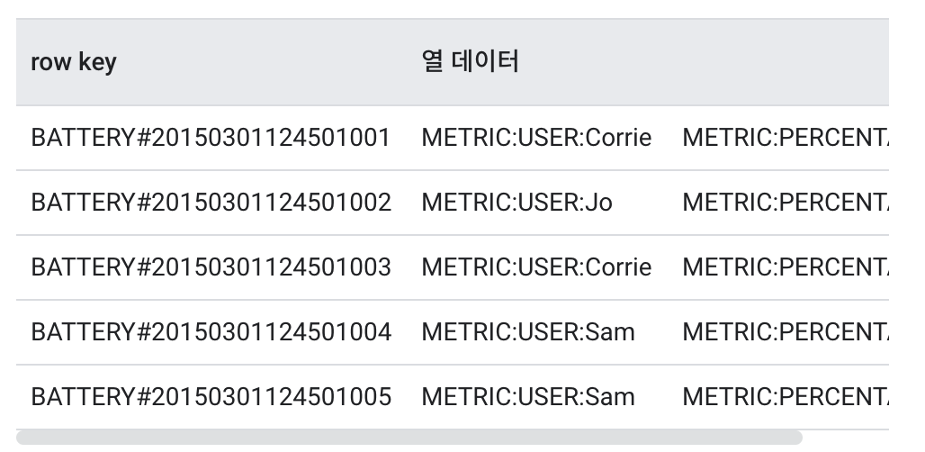
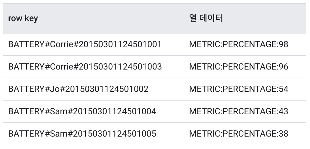
Filed Promotion
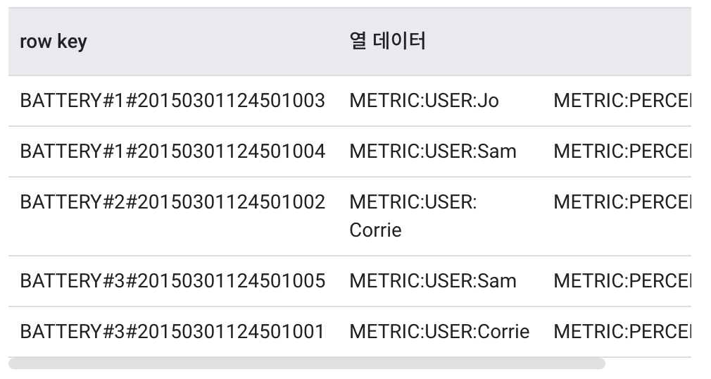
Sorting
Hash divided as 3 because predicted number of clusters is 3.
 ![]
![]
By default, field promotion is better. Field promotions prevent hotspot formation in almost any case and make it easier to design rowkeys to facilitate querying.Use sorting only if field promotion does not solve the load concentration problem.
6.2. DataBase Test
- Create a table using the column family and column qualifiers that you created for the schema.
- Load a table with at least 30GB of test data using the rowkey identified by the temporary plan. Keep below the storage usage limit per node.
- Run a test that experiences excessive load for several minutes. This step allows Cloud Bigtable to equalize data across nodes based on observed access patterns.
- Typically, you run an hour simulation of reads and writes to a table.
- Review the simulation results using Key Visualizer and Cloud Monitoring.
7. Instance management
7.1. SSD or HDD
When you create a Cloud Bigtable instance, select whether the cluster stores data on solid state drives (SSDs) or hard disk drives (HDDs). In most cases, SSD storage is the most efficient and cost-effective choice. HHD repositories are sometimes suitable for latency-sensitive, infrequently accessed, and extremely large datasets of more than 10TB.
Select SSD storage if unsure
SSDs are much faster and more predictable than HDDs. HDD throughput is much more limited than SSD throughput. HDDs are very slow to read individual rows. Unless you store a very large amount of data, there is no significant difference between the cost of using HDDs and the cost of Cloud Bigtable cluster nodes. Therefore, it is usually not recommended to use HDD storage unless you store more than 10TB of data.
Use cases where HDD storage is appropriate
You expect to store more than 10TB of data You are not planning to use data to support applications that are visible to you or that are latency sensitive. Batch operations that perform searches and writes and randomly read only occasionally a small number of rows; write very large amounts of data and keep very rarely read.
Transition to SSD and HDD storage
When you create a Cloud Bigtable instance and cluster, you cannot reverse the SSD or HDD storage that you select for the cluster. You cannot use Google Cloud Console to change the type of storage used in the cluster.
If you need to convert an existing HDD cluster to SSD, or vice versa, you need to export data from an existing instance and import data into a new one. Alternatively, you can copy data from one instance to another using Dataflow or Hadoop MapReduce operations. Because migrating the entire instance takes time, you might need to add nodes to the Cloud Bigtable cluster before migrating the instance.
Reference
[1] https://cloud.google.com/bigtable/docs
[2] https://bcho.tistory.com/1217