머신 러닝 - 모델 평가

◾모델 평가

• [데이터 수집/가공/변환 -> 모델 학습/예측 -> 모델 평가] 과정 반복
• 대부분 다양한 모델, 다양한 파라미터를 두고, 상대적으로 비교한다.
• 회귀 모델의 경우 : 실제 값과 에러치를 가지고 계산
  • 예측 결과 : 연속된 수치
• 분류 모델의 경우 : 정확도(Accuracy), 오차행렬(Confusion Matrix), 정밀도(Precision), 재현율(Recall), F1 score, ROC AUC 등
  • 예측 결과 : 몇 개의 종류(분류) 중 결과를 선택
  • IRIS, 타이타닉 등
• 이진 분류 모델의 경우
  • TP True Positive : 실제 Positive를 Positive라고 맞춘 경우
  • FN False Negative : 실제 Positive를 Negative라고 틀리게 예측한 경우
  • TN True Negative : 실제 Negative를 Negative라고 맞춘 경우
  • FP False Positive : 실제 Negative를 Positive라고 틀리게 예측한 경우
  • Accuracy(전체 데이터 중 맞게 예측한 비율) : ${TP + TN}\over{TP + TN + FP + FN}$
  • Precision(양성이라고 예측한 것 중 실제 양성의 비율) : ${TP}\over{TP + FP}$
  • RECALL(참인 데이터들 중에서 참이라고 예측한 것, TPR : True Positive Ratio) : ${TP} \over {TP+FN}$
  • FALL-OUT(실제 양성이 아닌데, 양성이라고 잘못 예측한 경우, FPR : False Position Ratio) : ${FP} \over {TN+FP}$
  • 예측 결과 : 2개의 종류 중 결과 선택

---

◾이진 모델 분류

• 분류 모델은 결과를 속할 비율(확률)로 반환
  • 지금까지는 비율의 threshold를 0.5로 하여 0, 1 반환(if 이진 분류)
  • iris의 경우 가장 높은 확률값이 있는 클래스를 결과로 반환
• threshold를 변경해가며 지표 관찰
  • Recall, Fall-out, Precision, Accuracy
  • threshold = 0.3, TP = 3, FN = 0, FP = 4, TN = 0

y	y_pred	output for threshold 0.3	Recall	Fall-out	Precision	Accuracy
0	0.4	1	3/3	4/4	3/7	3/7
1	0.9	1
0	0.3	1
1	0.8	1
1	0.4	1
0	0.5	1
0	0.6	1

• threshold = 0.4, TP = 3, FN = 0, FP = 3, TN = 1

y	y_pred	output for threshold 0.4	Recall	Fall-out	Precision	Accuracy
0	0.4	1	3/3	3/4	3/6	4/7
1	0.9	1
0	0.3	0
1	0.8	1
1	0.4	1
0	0.5	1
0	0.6	1

• threshold = 0.5, TP = 2, FN = 1, FP = 2, TN = 2

y	y_pred	output for threshold 0.5	Recall	Fall-out	Precision	Accuracy
0	0.4	0	2/3	2/4	2/4	4/7
1	0.9	1
0	0.3	0
1	0.8	1
1	0.4	0
0	0.5	1
0	0.6	1

• threshold = 0.6, TP = 2, FN = 1, FP = 1, TN = 3

y	y_pred	output for threshold 0.6	Recall	Fall-out	Precision	Accuracy
0	0.4	0	2/3	1/4	2/3	5/7
1	0.9	1
0	0.3	0
1	0.8	1
1	0.4	0
0	0.5	0
0	0.6	1

• threshold = 0.8, TP = 2, FN = 1, FP = 0, TN = 4

y	y_pred	output for threshold 0.8	Recall	Fall-out	Precision	Accuracy
0	0.4	0	2/3	0/4	2/2	6/7
1	0.9	1
0	0.3	0
1	0.8	1
1	0.4	0
0	0.5	0
0	0.6	0

• threshold = 0.9, TP = 1, FN = 2, FP = 0, TN = 4

y	y_pred	output for threshold 0.9	Recall	Fall-out	Precision	Accuracy
0	0.4	0	1/3	0/4	1/1	5/7
1	0.9	1
0	0.3	0
1	0.8	0
1	0.4	0
0	0.5	0
0	0.6	0

• Threshold 정리

	0.3	0.4	0.5	0.6	0.8	0.9
Recall	1.00	1.00	0.67	0.67	0.67	0.33
Precision	0.43	0.50	0.50	0.67	1.00	1.00
Fall-out	1.00	0.75	0.50	0.25	0.00	0.00
Accuracy	0.43	0.57	0.57	0.71	0.86	0.71

• Recall : 참인 데이터 중에서 참이라고 예측한 데이터의 비율
• Precision : 참이라고 예측한 것 중에서 실제 참인 데이터의 비율
• 실제 양성인 데이터를 음성이라고 판단하면 안되는 경우라면, Recall이 중요하고 이 경우 Threshold를 0.3 혹은 0.4로 선정(예 - 질병 확인)
• 실제 음성인 데이터를 양성이라고 판단하면 안되는 경우라면, Precision이 중요하고, 이 경우는 Threshold를 0.8 혹은 0.9로 선정(예 - 스팸 메일)
• Recall, Precision은 서로 영향을 주기 떄문에 한 쪽을 극단적으로 높게 설정하면 안된다.

---

◾F1-Score

• F1-Score(조화 평균) : Recall과 Precision을 결합한 지표
  • Recall과 Precision이 어느 한쪽으로 치우치지 않고 둘다 높은 값을 가질 수록 높은 값을 가진다.
  • $F_{\beta}~=~(1+\beta^{2})(\mathrm{precision}\times \mathrm{recall})/(\beta^{2}\mathrm{precision}+\mathrm{recall})$
  • F-Score에서 beta를 1로 두면 F1-Score
    • $F_{1}~=~2(\mathrm{precision}\times \mathrm{recall})/(\mathrm{precision}+\mathrm{recall})$
  • Threshold 정리

  	0.3	0.4	0.5	0.6	0.8	0.9
  Recall	1.00	1.00	0.67	0.67	0.67	0.33
  Precision	0.43	0.50	0.50	0.67	1.00	1.00
  Fall-out	1.00	0.75	0.50	0.25	0.00	0.00
  Accuracy	0.43	0.57	0.57	0.71	0.86	0.71
  F1-Score	0.60	0.67	0.57	0.67	0.80	0.50

---

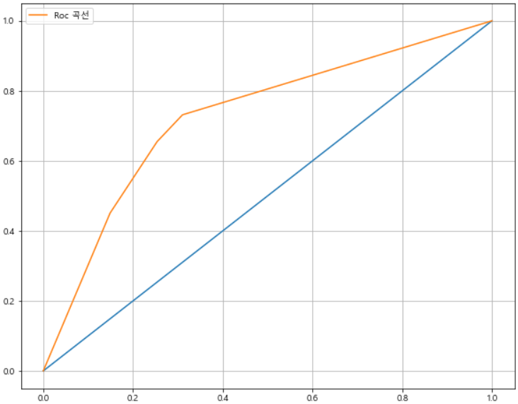
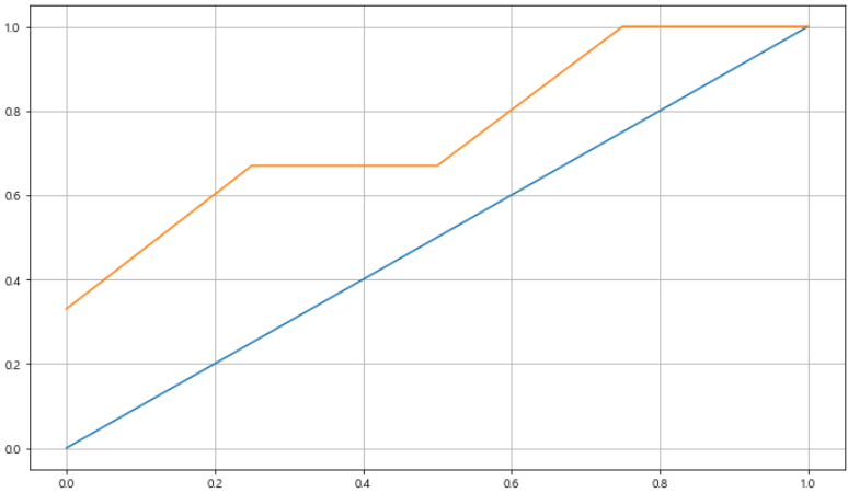
◾ROC와 AUC

• ROC : 분류 검정의 민감도 대 (1 - 특이도)를 도표화하여 모형 예측의 정확도를 평가하기 위한 유용한 방법
• AUC : ROC 곡선의 면적을 의미한다.
  
  • FPR(False Positive Rate)이 변할 때, TPR(True Positive Rate)의 변화를 그린 그림
  • FPR을 x축, TPR을 y축으로 놓고 그림
  • TPR은 Recall(Sensitivity : 민감도), FPR은 Fall-out
  • 직선에 가까울 수록 머신 러닝 모델의 성능이 떨어지는 것으로 판단(AUC = 0.5)
    
  • 수직에 가까울 수록 높은 성능을 의미한다.
    • 수직일 경우 AUC = 1
  • 위의 예제에서의 ROC 곡선
    • Fall-out이 같을 경우 Recall이 작은 것을 선택한다.
    • AUC는 1에 가까울 수록 좋은 수치로 0.5보다 커야한다.
    • recall = [1., 1., 0.67, 0.67, 0.67, 0.33]
    • fall-out = [1., 0.75, 0.5, 0.25, 0., 0.]
      • 4번째 요소와 5번째 요소의 fall-out이 같으므로 작은 값이 5번째 요소만 사용한다.

---

◾ROC 커브 그리기

• 와인 데이터를 이용해 Roc 커브 그리기

# 와인 ROC 곡선
# 와인 데이터 정리
import pandas as pd

red_wine = pd.read_csv('winequality-red.csv', sep=';')
white_wine = pd.read_csv('winequality-white.csv', sep=';')

red_wine['color'] = 1
white_wine['color'] = 0

wine = pd.concat([red_wine, white_wine])
wine.reset_index(drop=True, inplace=True)
wine['taste'] = [1. if grade > 5 else 0. for grade in wine['quality']]

X = wine.drop(['taste', 'quality'], axis=1)
y = wine['taste']

# Decision Tree 생성
from sklearn.model_selection import train_test_split
from sklearn.tree import DecisionTreeClassifier
from sklearn.metrics import accuracy_score

X_train, X_test, y_train, y_test = train_test_split(X, y, test_size=0.2, random_state=13)

wine_tree = DecisionTreeClassifier(max_depth=2, random_state = 13)
wine_tree.fit(X_train, y_train)

y_pred_tr = wine_tree.predict(X_train)
y_pred_test = wine_tree.predict(X_test)

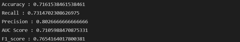
print("Train Acc : {}".format(accuracy_score(y_train, y_pred_tr)))
print("Test Acc : {}".format(accuracy_score(y_test, y_pred_test)))

# 각 수치 계산
from sklearn.metrics import accuracy_score, precision_score, recall_score, f1_score, roc_auc_score, roc_curve

print('Accuracy : {}'.format(accuracy_score(y_test, y_pred_test)))
print('Recall : {}'.format(recall_score(y_test, y_pred_test)))
print('Precision : {}'.format(precision_score(y_test, y_pred_test)))
print('AUC Score : {}'.format(roc_auc_score(y_test, y_pred_test)))
print('F1_score : {}'.format(f1_score(y_test, y_pred_test)))

# ROC 커브 그리기
import matplotlib.pyplot as plt
import set_matplotlib_korean

pred_proba = wine_tree.predict_proba(X_test)[:, 1]
fpr, tpr, threshols = roc_curve(y_test, pred_proba)

plt.figure(figsize=(10, 8))
plt.plot([0, 1], [0, 1])
plt.plot(fpr, tpr, label='Roc 곡선')
plt.legend()
plt.grid()
plt.show()