💡 Clustering

Group a set of data points into clusters, where points in the same cluster are more similar to each other than to those in other clusters.

---

K-Means

• Definition : Clustering based on Centroid
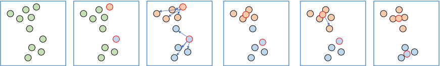  Set Two Centroid(Orange/Blue)
  -> Each data point is assigned to the nearest centroid
  -> Move the centroids to the mean position of the data points assigned to them
  -> Each data point is assigned to the nearest centroid based on the moved centroids
  -> Move the centroids again to the mean position of the data points assigned to them.
• Benefits
  • The most commonly used algorithm in general clustering, simple and straightforward
  • Applicable to large datasets
• Drawbacks
  • As a distance-based algorithm, clustering accuracy decreases significantly when the number of features is very high -> PCA is necessary
  • Performance time slows down with a high number of iterations
  • Vulnerable to outliers
• Sklearn KMeans Class Parameter
  • n_clusters : Specify the number of clusters, i.e., the number of cluster centroids
  • max_iter : Maximum number of iterations for centroid movement
  • labels_ : Labels of the cluster centroids to which each data point belongs
  • cluster_centers : Coordinates of each centroid

Mean Shift Clustering

• Perform clustering by using KDE (Kernel Density Estimation) to move data points towards areas of high data density.
• Do not specify the number of clusters separately; the number of clusters is automatically determined based on the data distribution.
• When a specific data point moves to the location with the highest probability density within a radius, input the distance values to surrounding data points into the kernel function, then update and move the data point based on the returned value from its current position.
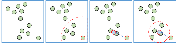  Original data
  -> Calculate the data distribution by including surrounding data within a specific radius for each individual data point
  -> Move the centroid towards the direction of higher data density
  -> Recalculate the data distribution within the radius from the moved data points
• KDE(Kernerl Density Estimation) : A method of estimating the probability density function of a random variable through a kernel function.
  • Estimate the probability density function by applying the kernel function to each observed data point, summing all the values, and then dividing by the number of data points.
  • Probability Density Function (PDF): A function that represents the distribution of a random variable, e.g., normal distribution, gamma distribution, t-distribution, etc.
  • Methods of Probability Density Estimation
    • Parametric Estimation: A method of finding the data distribution under the assumption that the data follows a specific distribution, e.g., Gaussian Mixture
    • Non-Parametric Estimation: A method of estimating density without assuming the data follows a specific distribution, finding the probability density based solely on the observed data, e.g., KDE
  • Changes in KDE according to bandwidth
    
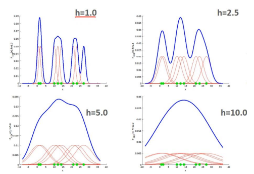
    • As the bandwidth (h) value decreases, the KDE becomes narrow and sharp, resulting in an estimated probability density function with high variability (Overfitting).
    • As the bandwidth (h) value increases, the KDE becomes excessively smooth, resulting in an overly simplified estimated probability density function (Underfitting).
      
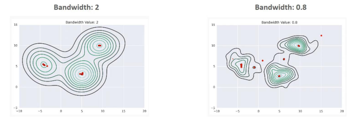
    • As the bandwidth increases, the number of clustering centroids decreases; as the bandwidth decreases, the number of clustering centroids increases.
    • Mean Shift performs clustering without specifying the number of clusters, with the number of clusters depending on the size of the bandwidth.
• Sklearn Mean Shift Parameter
  • bandwidth : A parameter that determines the width of the kernel function
  • estimate_bandwidth() : Functions provided for calculating the optimal bandwidth

GMM

• K-Means is effective for clustering datasets that are spread out around specific centroids, as shown on the left, but it is less efficient for clustering datasets like the one on the right.
  
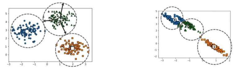
• Definition : Assume that the data to be clustered follows multiple different Gaussian distributions and perform clustering accordingly. ex) if there are 1,000 data points, extract several normal distribution curves that make up the data and determine which normal distribution each individual data point belongs to.
• EM for GMM parameter estimation(Expectation and Maximization)
  • Expectation : For each individual data point, calculate the probability of belonging to each specific normal distribution and assign it to the normal distribution with the highest probability (initially, randomly assign data points to specific normal distributions).
  • Maximization : Once the data points are assigned to a specific normal distribution, recalculate the mean and variance of that normal distribution. Then, determine the mean and variance (parameters) such that the likelihood of observing the given data is maximized (Maximum Likelihood).
  • If the mean and variance of the individual normal distributions no longer change and the assignments of the individual data points to the normal distributions no longer change, the final clustering is determined. Otherwise, continue repeating the Expectation and Maximization steps.
• Sklearn GaussianMixture Parameter
  • n_components : The number of mixture models, i.e., the number of clusters.

DBSCAN

• Definition : Based on an algorithm that relies on differences in data density within a specific space, it can perform clustering well even on datasets with geometric distributions.
• Characteristics
  • Since the algorithm automatically detects differences in data density to create clusters, the user cannot specify the number of clusters.
  • If the data density changes frequently or if the density of all data points does not vary significantly, the clustering performance will decrease.
  • If the number of features is large, the clustering performance will decrease..
• Components
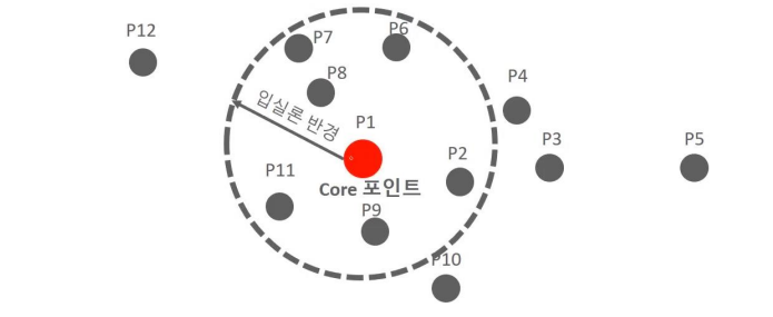
  • epsilon : A circular area with an epsilon radius centered on each individual data point.
  • min points : The number of other data points included in the epsilon neighborhood of each individual data point.
  • Core Point : If a data point has other data points within its neighborhood equal to or exceeding the minimum number of data points, that data point
  • Neighbor Point : Other data points located within the neighborhood
  • Border Point : Data points that do not have at least the minimum number of neighboring points within the neighborhood but have a core point as a neighboring point
  • Noise Point : Data points that do not have at least the minimum number of neighboring points within the neighborhood and do not have a core point as a neighboring point
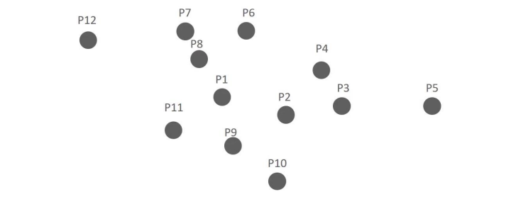
• DBSCAN PROCEDURE
  1. Example of applying DBSCAN to a dataset of 12 data points from P1 to P12, assuming the minimum number of data points to be included within a specific epsilon radius, including the point itself, is 6.
     
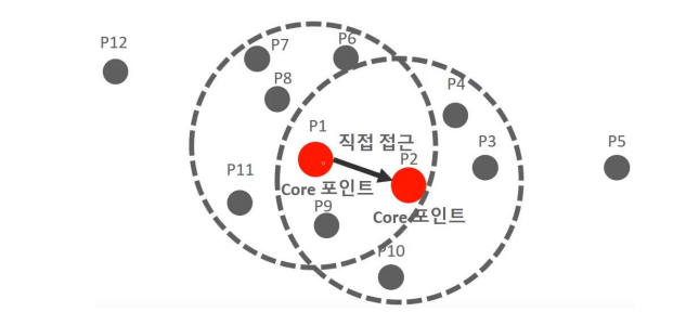
  2. Based on the P1 data point, there are 7 data points within the epsilon radius (including P1 itself, and neighboring points P2, P6, P7, P8, P9, P11). Since this satisfies the minimum requirement of 6 data points, the P1 data point becomes a core point.
     
  3. The P2 data point also has 6 data points within the radius (P2, P1, P3, P4, P9, P10), so it becomes a core point.
     
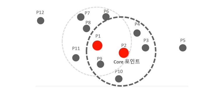
  4. If the neighboring data point P2 of core point P1 is also a core point, it can be directly accessed from P1 to P2.
     
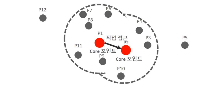
  5. Form clusters by connecting other core points that can be directly accessed from a specific core point -> Gradually expand the cluster area using this method.
     
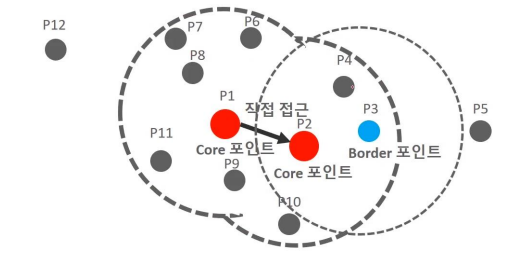
  6. In the case of P3, the neighboring data points within the radius are P2 and P4, so it cannot be a core point. However, it has a neighboring core point, P2. -> Data points that are not core points but have a neighboring core point are called border points.
     
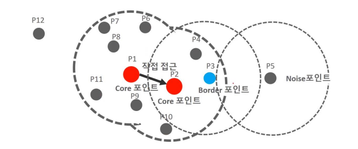
  7. Data points like P5 that do not have the minimum number of neighboring data points within the radius and do not have a core point as a neighboring data point are called Noise Points.
     
• Sklearn DBSCAN parameter
  • eps : Radius of the epsilon neighborhood.
  • min_samples : The minimum number of data points that must be included within the epsilon neighborhood for a point to become a core point. Including the data point itself, this becomes min_samples + 1.

Clustering Performance Evaluation

Silhouette Analysis

• Definition
  • Indicate how efficiently the clusters are separated from each other
  • Based on the Silhouette Coefficient, which is an individual clustering metric for each data point
• Silhouette Coeffieicnt : A metric that indicates how closely a data point is clustered with other points in the same cluster and how far it is separated from points in other clusters
  
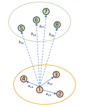
  • $a_{ij}$ : The distance from the $i$th data point to other data points within the same cluster. For example, $a_{12}$ is the distance from data point 1 to data point 2
  • $a_i$ : The average distance from the $i$th data point to other data points within the same cluster. For example, $a_i$ = average($a_{12}$, $a_{13}$, $a_{14}$)
  • $b_i$ : The average distance from the $i$th data point to the data points in the nearest other cluster. For example, $b_i$ = average($b_{15}$, $b_{16}$, $b_{17}$, $b_{18}$)
    
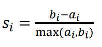
  • The value indicating how far apart two clusters are is $b_i-a_i$ and to normalize this value, it is divided by $max(a_i, b_i)$
  • The Silhouette Coefficient ranges from -1 to 1. The closer it is to 1, the further the data point is from neighboring clusters. The closer it is to 0, the closer the data point is to neighboring clusters. A negative value indicates that the data point has been assigned to the wrong cluster.
• Sklearn silhoueet_samples : By inputting the X feature dataset and the cluster label data (labels) that each feature dataset belongs to as arguments, it returns the Silhouette Coefficient for each data point.
• Sklearn silhoueet_score : By inputting the X feature dataset and the cluster label data (labels) that each feature dataset belongs to as arguments, it calculates and returns the average Silhouette Coefficient of the entire dataset.
  • A good clustering criterion based on silhouette analysis is when the value of the silhouette_score function is between 0 and 1, with values closer to 1 being better.
  • However, in addition to the average Silhouette Coefficient of the entire dataset, the deviation of the average values of individual clusters should not be large. In other words, it is important that the average Silhouette Coefficient of individual clusters does not deviate significantly from the overall average Silhouette Coefficient.