Uplift package scikit-uplift 예제를 보며 알아보는 시간

https://github.com/maks-sh/scikit-uplift

https://colab.research.google.com/github/maks-sh/scikit-uplift/blob/master/notebooks/RetailHero_EN.ipynb#scrollTo=olRc5k9iCIMP

Introduction

Before proceeding to the discussion of uplift modeling, let's imagine some situation:

A customer comes to you with a certain problem: it is necessary to advertise a popular product using the sms. You know that the product is quite popular, and it is often installed by the customers without communication, that the usual binary classification will find the same customers, and the cost of communication is critical for us...

어떤 유명한 상품을 sms를 통해 광고하려고 한다.
이 상품은 꽤 유명하고 소통(광고?) 없이도 자주 설치되었고 전통적인 확률 모델로는 같은 고객을 찾을 것이고 가성비있는 광고를 하고 싶다.

And then you begin to understand that the product is already popular, that the product is often installed by customers without communication, that the usual binary classification will find many such customers, and the cost of communication is critical for us...

그리고나서 깨닫는게
이 상품은 이미 유명하고 자주 설치했던 사람들을 대상으로 확률을 높게 부여할 것인데 이게 과연 가성비에 맞는가? 싶은 사실을 알게 된다.

= 전통적인 확률 모델로는 고객들을 세그먼트 하지 않는다.
= 흔히 업리프트 모델에선 고객을 4가지로 분류하는데, 우리의 핵심 타겟은 광고로 인하여 반응할 확률이 높은 고객들이다.

또 언급되는 4가지 분류

• Do-Not-Disturbs (a.k.a. Sleeping-dogs)
  have a strong negative response to a marketing communication. They are going to purchase if NOT treated and will NOT purchase IF treated. It is not only a wasted marketing budget but also a negative impact. For instance, customers targeted could result in rejecting current products or services. In terms of math: Wi=1,Yi=0 or Wi=0,Yi=1 .
  = treat를 했을때 반응을 안했거나 treat를 안했음에도 반응한 사람들

• Lost Causes
  will NOT purchase the product NO MATTER they are contacted or not. The marketing budget in this case is also wasted because it has no effect. In terms of math: Wi=1,Yi=0 or Wi=0,Yi=0 .
  = treat를 하건 안하건 반응을 하지 않는 사람들

• Sure Things
  will purchase ANYWAY no matter they are contacted or not. There is no motivation to spend the budget because it also has no effect. In terms of math: Wi=1,Yi=1 or Wi=0,Yi=1 .
  = treat를 하건 안하건 반응을 하는 사람들

• Persuadables
  will always respond POSITIVE to the marketing communication. They is going to purchase ONLY if contacted (or sometimes they purchase MORE or EARLIER only if contacted). This customer's type should be the only target for the marketing campaign. In terms of math: Wi=0,Yi=0 or Wi=1,Yi=1 .
  = treat를 안했을땐 반응을 하지만 teat를 했을때 반응한 사람들 !!

Because we can't communicate and not communicate with the customer at the same time, we will never be able to observe exactly which type a particular customer belongs to.
= 저번 글에서도 같은 내용이 있었음
= 각 개인이 정확히 어떻게 행동할지는 모름

Depends on the product characteristics and the customer base structure some types may be absent. In addition, a customer response depends heavily on various characteristics of the campaign, such as a communication channel or a type and a size of the marketing offer. To maximize profit, these parameters should be selected.

고객들 반응은 주로 캠페인의 성격에 따라 다양하게 달라지고
( 캠페인의 성격 : 커뮤니케이션 되었던 채널이나 마케팅의 사이즈, 타입(?) )

이익을 극대화하기 위해선 이러한 파라미터가 설정되야만 한다.

Thus, when predicting uplift score and selecting a segment by the highest score, we are trying to find the only one type: persuadables.

Thus, in this task, we don’t want to predict the probability of performing a target action, but to focus the advertising budget on the customers who will perform the target action only when we interact.

In other words, we want to evaluate two conditional probabilities separately for each client:

따라서 반응할 확률을 예측하기보다
우리가 관심있는 그룹이 반응할 확률에 집중(예측)해야 한다.

다른 말로, 2가지의 조건부 확률을 각 고객에 대해서 평가하려고 한다.

Performing a targeted action when we influence the client. We will refer such clients to the test group (aka treatment): PT=P(Y=1|W=1) ,

고객에게 광고했을때 반응했다면 이러한 고객들은 테스트 그룹(treatment)이라고 명칭(명명)한다.

Performing a targeted action without affecting the client. We will refer such clients to the control group (aka control): PC=P(Y=1|W=0) ,

고객에게 광고를 하지 않았을때 반응했다면 이러한 고객들은 컨트롤 그룹(control)이라고 명명한다.

where Y is the binary flag for executing the target action, and W is the binary flag for communication (in English literature, treatment)

여기서 Y 는 1,0 의 바이너리 값이다. 반응 유무.
여기서 W 는 1,0 의 바이너리 값이다. 조치(treatment,변인,광고) 유무.

The very same cause-and-effect effect is called uplift and is estimated as the difference between these two probabilities:

매우 동일한 원인과 결과의 효과를 uplift 라고 하며, 2가지 확률의 차이로 구할 수 있다.

uplift=P.T−P.C=P(Y=1|W=1)−P(Y=1|W=0)

Predicting uplift is a cause-and-effect inference task.
The point is that you need to evaluate the difference between two events that are mutually exclusive for a particular client (either we interact with a person, or not; you can't perform two of these actions at the same time).

핵심은 실험자는 각 개인의 상호 베타적인 (독립적인) 2개 이벤트(P.t, P.c)의 차이를 계산해야 한다. ( 우리가 사람과 상호 작용하든 그렇지 않든, 이 두 가지 작업을 동시에 수행할 수는 없습니다.)
= ( 실제로는 동일한 사람에게 동일한 A/B 테스팅을 독립적으로 2번 시행할 수 없다. )

This is why additional requirements for source data are required for building uplift models.

이러한 점이 업리프트 모델을 만들때 추가 조건이 붙는 이유이다.

To get a training sample for the uplift simulation, you need to conduct an experiment:

업리프트 시뮬레이션을 하기 위해서 당신은 실험을 해야만 한다.

1. Randomly split a representative part of the client base into a test and control group
   랜덤하게 고객을 테스트 그룹과 컨트롤 그룹으로 분리해야 한다.
   ( 테스트 그룹 : 고객에게 광고했을때 반응하는 그룹
   컨트롤 그룹 : 고객에게 광고를 하지 않았을때 반응하는 그룹 )

2. Communicate with the test group

The data obtained as part of the design of such a pilot will allow us to build an uplift forecasting model in the future.
It is also worth noting that the experiment should be as similar as possible to the campaign, which will be launched later on a larger scale.

이러한 파일럿 설계의 일부로 얻은 데이터를 통해 향후 상승 예측 모델을 구축할 수 있습니다.
또한 실험은 나중에 더 큰 규모로 시작될 캠페인과 최대한 유사해야 한다는 점도 주목할 가치가 있습니다.

The only difference between the experiment and the campaign should be the fact that during the pilot, we choose random clients for interaction, and during the campaign - based on the predicted value of the Uplift.
If the campaign that is eventually launched differs significantly from the experiment that is used to collect data about the performance of targeted actions by clients, then the model that is built may be less reliable and accurate.

실험과 캠페인의 유일한 차이점은 파일럿 중에 상호 작용을 위해 무작위 클라이언트를 선택하고 캠페인 중에 Uplift의 예측 값을 기반으로 한다는 사실입니다.

최종적으로 실행되는 캠페인이 고객이 목표로 하는 행동의 성과에 대한 데이터를 수집하는 데 사용되는 실험과 크게 다른 경우 구축된 모델은 덜 안정적이고 정확하지 않을 수 있습니다.

So, the approaches to predicting uplift are aimed at assessing the net effect of marketing campaigns on customers.

All classical approaches to uplift modeling can be divided into two classes:

1. Approaches with the same model
2. Approaches using two models

업리프트 모델링의 방법론은 2가지로 나뉜다.

1. 하나의 모델로 접근
2. 2개의 모델로 접근

---

1. Single model approaches

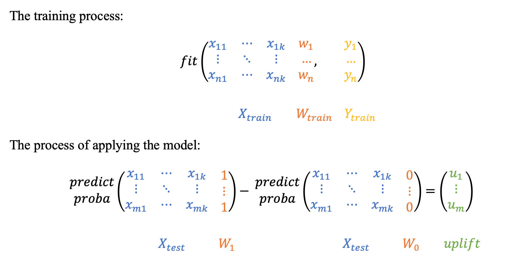
1.1 Single model with treatment as feature

The most intuitive and simple uplift modeling technique.

가장 단순하면서 직관적인 방법이다.

A training set consists of two groups: treatment samples and control samples.

학습 데이터 셋은 2개의 그룹으로 구성되어 있다.

조치를 받은 그룹과 컨트롤 받은 그룹

( 테스트 그룹 : 고객에게 광고했을때 반응하는 그룹
컨트롤 그룹 : 고객에게 광고를 하지 않았을때 반응하는 그룹 )

a | b | a | c | 0 | --- | 1
b | b | a | b | 1 | --- | 0
a | a | b | c | 0 | --- | 1
b | a | b | b | 1 | --- | 0

이런 데이터가 있다면

하나의 모델로 학습 후,

테스트 데이터셋에서 treatment 를 각 1로 채운것과 0으로 채운 값의 차이를 구한다.

There is also a binary treatment flag added as a feature to the training set.

After the model is trained, at the scoring time it is going to be applied twice:

with the treatment flag equals 1 and with the treatment flag equals 0.

Subtracting these model's outcomes for each test sample, we will get an estimate of the uplift.

1.2 Class Transformation

Simple yet powerful and mathematically proven uplift modeling method, presented in 2012. The main idea is to predict a slightly changed target Zi :

Zi=Yi⋅Wi+(1−Yi)⋅(1−Wi),

where

Zi - new target variable of the i client;
Yi - target variable of the i client;
Wi - flag for communication of the i client;
In other words, the new target equals 1 if a response in the treatment group is as good as a response in the control group and equals 0 otherwise:

Zi=⎧⎩⎨1,1,0,if Wi=1 and Yi=1if Wi=0 and Yi=0otherwise

Let's go deeper and estimate the conditional probability of the target variable:

P(Z=1|X=x)==P(Z=1|X=x,W=1)⋅P(W=1|X=x)++P(Z=1|X=x,W=0)⋅P(W=0|X=x)==P(Y=1|X=x,W=1)⋅P(W=1|X=x)++P(Y=0|X=x,W=0)⋅P(W=0|X=x).

We assume that W is independent of X=x by design. Thus we have: P(W|X=x)=P(W) and

P(Z=1|X=x)==PT(Y=1|X=x)⋅P(W=1)++PC(Y=0|X=x)⋅P(W=0)

Also, we assume that P(W=1)=P(W=0)=12 , which means that during the experiment the control and the treatment groups were divided in equal proportions. Then we get the following:

P(Z=1|X=x)==PT(Y=1|X=x)⋅12+PC(Y=0|X=x)⋅12⇒2⋅P(Z=1|X=x)==PT(Y=1|X=x)+PC(Y=0|X=x)==PT(Y=1|X=x)+1−PC(Y=1|X=x)⇒⇒PT(Y=1|X=x)−PC(Y=1|X=x)==uplift=2⋅P(Z=1|X=x)−1

Thus, by doubling the estimate of the new target Z and subtracting one we will get an estimation of the uplift:

uplift=2⋅P(Z=1)−1

This approach is based on the assumption: P(W=1)=P(W=0)=12 , That is the reason that it has to be used only in cases where the number of treated customers (communication) is equal to the number of control customers (no communication).

2. Approaches with two models

The two-model approach can be found in almost any uplift modeling work and is often used as a baseline. However, using two models can lead to some unpleasant consequences: if you use fundamentally different models for training, or if the nature of the test and control group data is very different, then the scores returned by the models will not be comparable. As a result, the calculation of the uplift will not be completely correct. To avoid this effect, you need to calibrate the models so that their scores can be interpolated as probabilities. The calibration of model probabilities is described perfectly in scikit-learn documentation.

2.1 Two independent models
The main idea is to estimate the conditional probabilities of the treatment and control groups separately.

Train the first model using the treatment set.
Train the second model using the control set.
Inference: subtract the control model scores from the treatment model scores.

import sys

# install uplift library scikit-uplift and other libraries 
!{sys.executable} -m pip install scikit-uplift catboost pandas

from sklearn.model_selection import train_test_split
from sklift.datasets import fetch_x5
import pandas as pd

pd.set_option('display.max_columns', None)
%matplotlib inline

print(f"Dataset type: {type(dataset)}\n")
print(f"Dataset features shape: {dataset.data['clients'].shape}")
print(f"Dataset features shape: {dataset.data['train'].shape}")
print(f"Dataset target shape: {dataset.target.shape}")
print(f"Dataset treatment shape: {dataset.treatment.shape}")

ataset type: <class 'sklearn.utils.Bunch'>

Dataset features shape: (400162, 5)
Dataset features shape: (200039, 1)
Dataset target shape: (200039,)
Dataset treatment shape: (200039,)

# extract data

df_clients = dataset.data['clients'].set_index("client_id")
df_train = pd.concat([dataset.data['train'], dataset.treatment , dataset.target], axis=1).set_index("client_id")
indices_test = pd.Index(set(df_clients.index) - set(df_train.index))

# extracting features

df_features = df_clients.copy()

df_features['first_issue_time'] = \
    (pd.to_datetime(df_features['first_issue_date'])
     - pd.Timestamp('1970-01-01')) // pd.Timedelta('1s')
     
df_features['first_redeem_time'] = \
    (pd.to_datetime(df_features['first_redeem_date'])
     - pd.Timestamp('1970-01-01')) // pd.Timedelta('1s')
     
df_features['issue_redeem_delay'] = df_features['first_redeem_time'] \
    - df_features['first_issue_time']
    
df_features = df_features.drop(['first_issue_date', 'first_redeem_date'], axis=1)

indices_learn, indices_valid = train_test_split(df_train.index, test_size=0.3, random_state=123)

X_train = df_features.loc[indices_learn, :]
y_train = df_train.loc[indices_learn, 'target']
treat_train = df_train.loc[indices_learn, 'treatment_flg']

X_val = df_features.loc[indices_valid, :]
y_val = df_train.loc[indices_valid, 'target']
treat_val =  df_train.loc[indices_valid, 'treatment_flg']

X_train_full = df_features.loc[df_train.index, :]
y_train_full = df_train.loc[:, 'target']
treat_train_full = df_train.loc[:, 'treatment_flg']

X_test = df_features.loc[indices_test, :]

cat_features = ['gender']

models_results = {
    'approach': [],
    'uplift@30%': []
}