Data Visualization
3-3. Facet
1) Multiple View
Facet이란?
-
'분할'을 의미
-
화면 상에 View를 분할 및 추가하여 다양한 관점을 전달한다
-
같은 데이터 셋에 서로 다른 인코딩을 해서 다른 인사이트를 얻을 수도 있고,
-
같은 방법으로 동시에 여러 feature들을 보거나,
-
큰 틀에서 볼 수 없는 부분 집합을 세세하게 볼 때 facet을 사용한다.
2) Matplotlib으로 구현해보기
Figure & Axes
-
Figure은 큰 틀, Axes는 각 플롯이 들어가는 공간
-
Figure은 언제나 한 개, 플롯은 N개
- 필요한 라이브러리 가져오기
import numpy as np
import matplotlib as mpl
import matplotlib.pyplot as plt- Figure Color : 하얀 배경의 내용일 때 차트와 배경을 구분하기 위해 배경 색을 바꿀 수 있다
fig, ax = plt.subplots()
fig.set_facecolor('lightgray')
plt.show()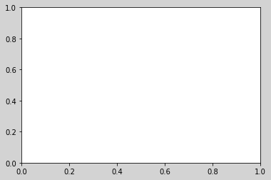
- figure에 subplot을 추가할 수 있는 쉬운 3가지 방법
- plt.subplot() : 현재 이미지 영역(fig=figure())에 추가
- plt.figure() + fig.add_subplot() (권장) : fig라는 객체 선택하여 거기에 서브플롯 추가
- plt.subplots() (권장) : 여러 개의 subplot추가
''' plt.subplot() '''

fig = plt.figure()
ax = plt.subplot(121)
ax = plt.subplot(122)
plt.show()

''' plt.figure() + fig.add_subplot() : 권장 '''

fig = plt.figure()
ax = fig.add_subplot(121)
ax = fig.add_subplot(122)
plt.show()
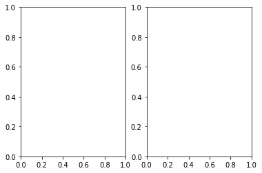
''' plt.subplots() : 권장 '''

fig, axes = plt.subplots(1, 2) # 세로 한 칸, 가로 두 칸
#fig, (ax1, ax2) = plt.subplots(1, 2)
plt.show()

Figure & Axes Properties
1) Figure Size : figure 크기, figsize로 조정한다. ( 이전에 많이 다뤘으므로 생략한다 )
2) DPI(dots per inch) : 해상도, 기본값은 100이다.
- 고해상도는 시간이 걸리니까 처음에는 저해상도로 작업하다가, 그래프를 저장할 때 고해상도로 저장하자
- 일반 해상도 그래프
fig = plt.figure()
ax1 = fig.add_subplot(121)
ax2 = fig.add_subplot(122)
ax1.plot([1, 2, 3], [1, 4, 9])
ax2.plot([1, 2, 3], [1, 2, 3])
plt.show()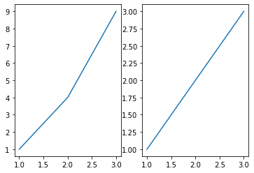
- 고해상도 그래프(좀 더 선명해지고, 크기도 좀 더 커지는 것을 볼 수 있다.)
fig = plt.figure(dpi=150)
ax1 = fig.add_subplot(121)
ax2 = fig.add_subplot(122)
ax1.plot([1, 2, 3], [1, 4, 9])
ax2.plot([1, 2, 3], [1, 2, 3])
plt.show()
- 해상도를 조절하여 저장할 수도 있다.
fig.savefig('file_name', pdi=150) # 해상도 조절하여 저장 가능3) Sharex, Sharey
- 개별 ax에 대해서나 subplots 함수를 사용할 깨는 sharew, sharey를 사용하여 축을 공유할 수 있다.
fig = plt.figure()
ax1 = fig.add_subplot(121)
ax1.plot([1, 2, 3], [1, 4, 9])
ax2 = fig.add_subplot(122, sharey=ax1) # ax1와 y축 공유
ax2.plot([1, 2, 3], [1, 2, 3])
plt.show()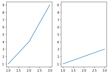
fig, axes = plt.subplots(1, 2, sharey=True) # 만드는 모든 subplots y축 공유

axes[0].plot([1, 2, 3], [1, 4, 9])
axes[1].plot([1, 2, 3], [1, 2, 3])
plt.show()
4) Squeeze
-
subplots()로 생성하면 기본적으로 다음과 같은 경우의 수로 서브플롯 ax 배열이 생성된다.
- 1 x 1 : 객체 1개(ax)
- 1 x N 또는 N x 1 : 길이가 N인 배열(axes[i])
- N x M : N by M 행렬(axes[i][j])
-
즉 plt.subplots()는 1차원을 제거하는 squeeze의 기본값이 True이기 때문에,
numpy ndarray에서 각각 차원이 0, 1, 2로 나타난다.
-
따라서 squeeze를 False로 두면 항상 2차원으로 배열을 받을 수 있고,
가변 크기에 대해 반복문을 사용하기 용이하다.
n, m = 1, 3

fig, axes = plt.subplots(n, m, squeeze=False, figsize=(m*2, n*2)) # 1차원 dim squeeze 하지 않는다
idx = 0
for i in range(n):
    for j in range(m):
        axes[i][j].set_title(idx)
        axes[i][j].set_xticks([])
        axes[i][j].set_yticks([])
        idx+=1

plt.show()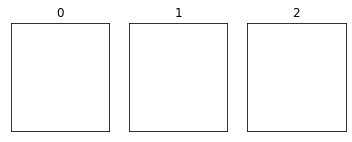
5) Flatten
- plt.subplots()나 plt.gca()로 받는 ax 리스트는 numpy ndarray로 전달되기 때문에, 1중 반복문을 쓰고 싶다면 flatten() 메서드를 사용할 수 있다.
n, m = 2, 3

fig, axes = plt.subplots(n, m, figsize=(m*2, n*2))

print(type(axes))
print(axes.shape)

for i, ax in enumerate(axes.flatten()): # 1중 반복문 사용을 위해 flatten 메소드 사용
    ax.set_title(i)
    ax.set_xticks([])
    ax.set_yticks([])


plt.show()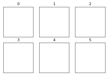
6) Aspect
- (y축 눈금(한 칸) 길이 / x축 눈금 길이) 값, 즉 x축 눈금 길이에 대한 y축 눈금 길이의 비율을 의미한다.
- aspect =1과 aspect=0.5 비교
fig = plt.figure(figsize=(12, 5))
ax1 = fig.add_subplot(121, aspect=1) # 세로 = 가로 * 1 (축 눈금 기준)
ax2 = fig.add_subplot(122, aspect=0.5) # 세로 = 가로 * 0.5 (축 눈금 기준)
plt.show()
- aspect =1과 aspect=0.5에서, aspect=0.5인 ax2에서 y축의 범위를 2배 늘렸을 때
( ax2의 y축 눈금 길이가 x축 눈금 길이의 0.5배인데 범위는 2배이므로 ax의 가로, 세로 길이 비율은 1 : 1)
fig = plt.figure(figsize=(12, 5))
ax1 = fig.add_subplot(121, aspect=1)
ax2 = fig.add_subplot(122, aspect=0.5) # 세로 = 가로 * 0.5 (축 눈금 기준)

ax2.set_xlim(0, 1)
ax2.set_ylim(0, 2)
plt.show()
Grid Spec
1) fig.add_gridspec()
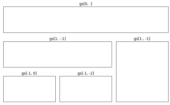
- N by M 그리드에서 슬라이싱을 이용해 서브플롯을 배치할 수 있다.
fig = plt.figure(figsize=(8, 5))

gs = fig.add_gridspec(3, 3) # make 3 by 3 grid (row, col)

ax = [None for _ in range(5)]

ax[0] = fig.add_subplot(gs[0, :])
ax[0].set_title('gs[0, :]')

ax[1] = fig.add_subplot(gs[1, :-1])
ax[1].set_title('gs[1, :-1]')

ax[2] = fig.add_subplot(gs[1:, -1])
ax[2].set_title('gs[1:, -1]')

ax[3] = fig.add_subplot(gs[-1, 0])
ax[3].set_title('gs[-1, 0]')

ax[4] = fig.add_subplot(gs[-1, -2])
ax[4].set_title('gs[-1, -2]')

for ix in range(5):
    ax[ix].set_xticks([])
    ax[ix].set_yticks([])

plt.tight_layout()
plt.show()
2) fig.subplot2grid()
-
N by M 그리드 시작점에서 delta x, delta y를 통해 표현할 수 있다.
-
fig.add_gridspec()과 같은 기능을 할 수 있지만, add_gridspec이 더 편리하다.
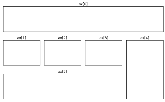
fig = plt.figure(figsize=(8, 5)) # initialize figure

ax = [None for _ in range(6)] # list to save many ax for setting parameter in each

ax[0] = plt.subplot2grid((3,4), (0,0), colspan=4)
ax[1] = plt.subplot2grid((3,4), (1,0), colspan=1)
ax[2] = plt.subplot2grid((3,4), (1,1), colspan=1)
ax[3] = plt.subplot2grid((3,4), (1,2), colspan=1)
ax[4] = plt.subplot2grid((3,4), (1,3), colspan=1,rowspan=2)
ax[5] = plt.subplot2grid((3,4), (2,0), colspan=3)


for ix in range(6):
    ax[ix].set_title('ax[{}]'.format(ix)) # make ax title for distinguish:)
    ax[ix].set_xticks([]) # to remove x ticks
    ax[ix].set_yticks([]) # to remove y ticks

fig.tight_layout()
plt.show()
Ax 내부에 서브 플롯 그리기
1) ax.inset_axes()
-
미니맵 등 원하는 서브플롯을 그릴 때 사용할 수 있다.
-
표현하고자하는 메인 시각화를 해치지 않는 선에서 사용하는 것을 추천한다.
fig, ax = plt.subplots()
axin = ax.inset_axes([0.8, 0.8, 0.2, 0.2]) # (0.8, 0.8) 위치에 0.2 x 0.2 플롯
plt.show()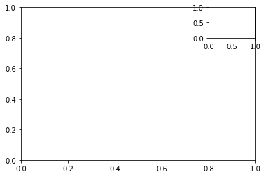
fig, ax = plt.subplots()

color=['royalblue', 'tomato']
ax.bar(['A', 'B'], [1, 2],
       color=color
      )

ax.margins(0.2)
axin = ax.inset_axes([0.8, 0.8, 0.2, 0.2])
axin.pie([1, 2], colors=color,
         autopct='%1.0f%%')
plt.show()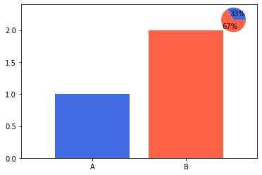
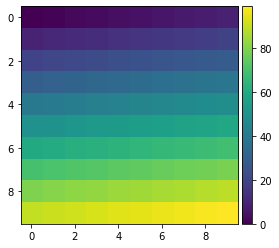
2) make_axes_locatable(ax)
-
그리드를 사용하지 않고 사이드에 추가하기
-
통계 정보를 제공할 수도 있고, 제목 등 텍스트 추가도 가능
-
일반적으로 colorbar에 가장 많이 사용됨
from mpl_toolkits.axes_grid1.axes_divider import make_axes_locatable

fig, ax = plt.subplots(1, 1)
ax_divider = make_axes_locatable(ax)

ax = ax_divider.append_axes("right", size="7%", pad="2%") # 오른쪽에, 전체 사이즈의 7% 크기로, 간격은 2%
plt.show()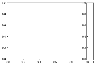
fig, ax = plt.subplots(1, 1)

# 이미지를 보여주는 시각화
# 2D 배열을 색으로 보여줌
im = ax.imshow(np.arange(100).reshape((10, 10)))

divider = make_axes_locatable(ax)
cax = divider.append_axes("right", size="5%", pad=0.05)

fig.colorbar(im, cax=cax)
plt.show()