[ML] Titanic 실습, labelencoder

Titinic

import pandas as pd

titanic = pd.read_excel('./titanic.xls')

import matplotlib.pyplot as plt
import seaborn as sns

titanic['survived'].value_counts() # 0: 생존x, 1: 생존

plot.pie, sns.countplot

titanic['survived'].value_counts().plot.pie();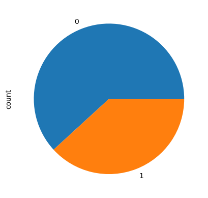

f, ax = plt.subplots(1, 2, figsize=(18, 8))

# 첫 번째 그림
titanic['survived'].value_counts().plot.pie(ax=ax[0], autopct='%1.1f%%', shadow=True, explode=[0, 0.05])
ax[0].set_title('Pie plot - survived')
ax[0].set_ylabel('')

# 두 번째 그림
sns.countplot(x='survived', data=titanic, ax=ax[1])
ax[1].set_title('Count plot - survived')

plt.show()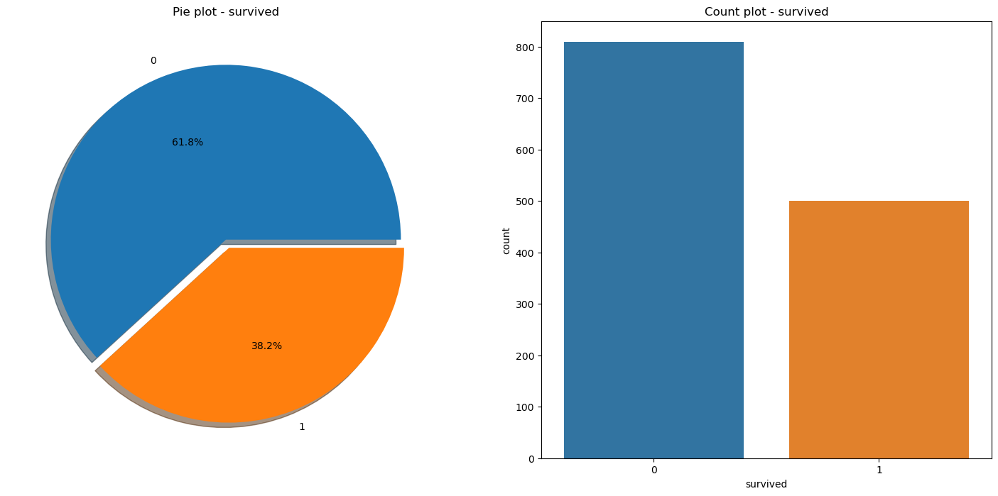

성별에 따른 생존 현황

f, ax = plt.subplots(1, 2, figsize=(18, 8))

# 첫 번째 그림
sns.countplot(x='sex', data=titanic, ax=ax[0])
ax[0].set_title('Count of passengers of sex')
ax[0].set_ylabel('')


# 두 번째 그림
sns.countplot(x='sex', data=titanic, hue='survived', ax=ax[1])
ax[1].set_title('Sex: survived and unsurvived')

plt.show()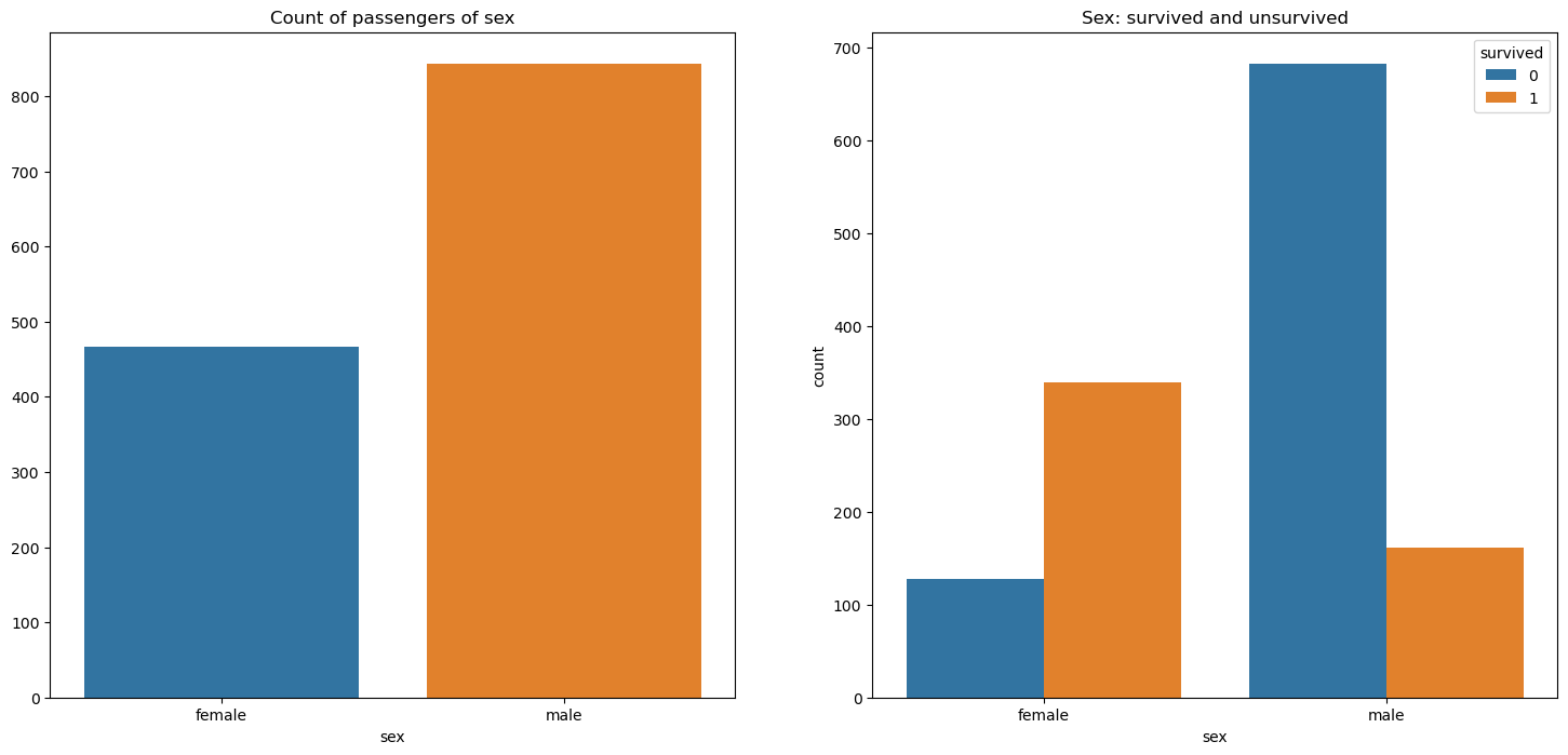

경제력 대비 생존률

sns.FacetGrid

pd.crosstab(titanic['pclass'], titanic['survived'], margins=True)  # margins=True: 합계 보여줌
# pclass: 1, 2, 3등실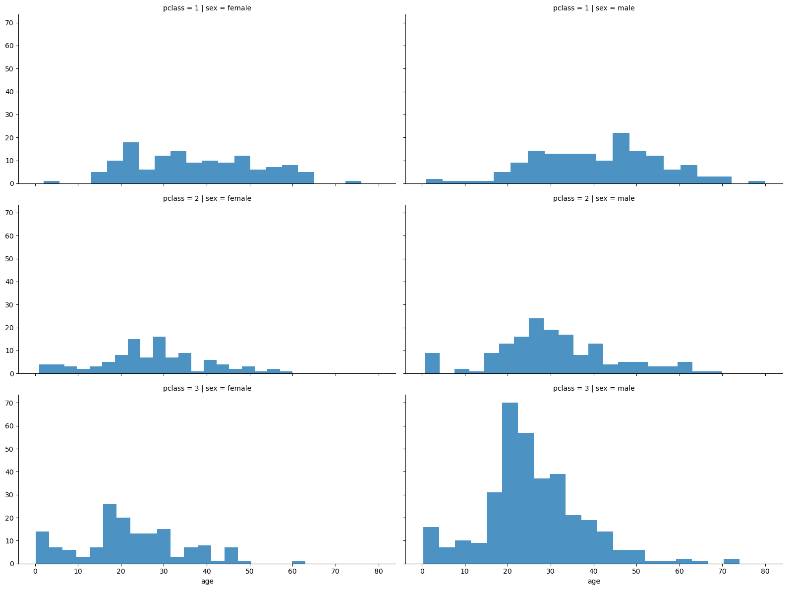

grid = sns.FacetGrid(titanic, row='pclass', col='sex', height=4, aspect=2)
grid.map(plt.hist, 'age', alpha=0.8, bins=20)
grid.add_legend();

3등실에는 남자가 많았음

px.histogram

import plotly.express as px

fig = px.histogram(titanic, x='age')
fig.show()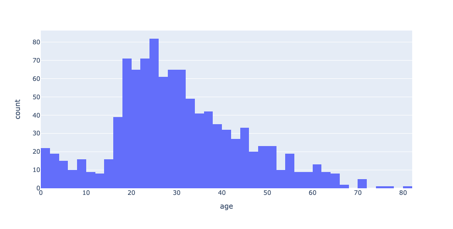

등실별 생존률 연령별로 관찰

plt.subplot, sns.barplot, sns.distplot

grid = sns.FacetGrid(titanic, col='survived', row='pclass', height=4, aspect=2)
grid.map(plt.hist, 'age', alpha=0.5, bins=20)
grid.add_legend();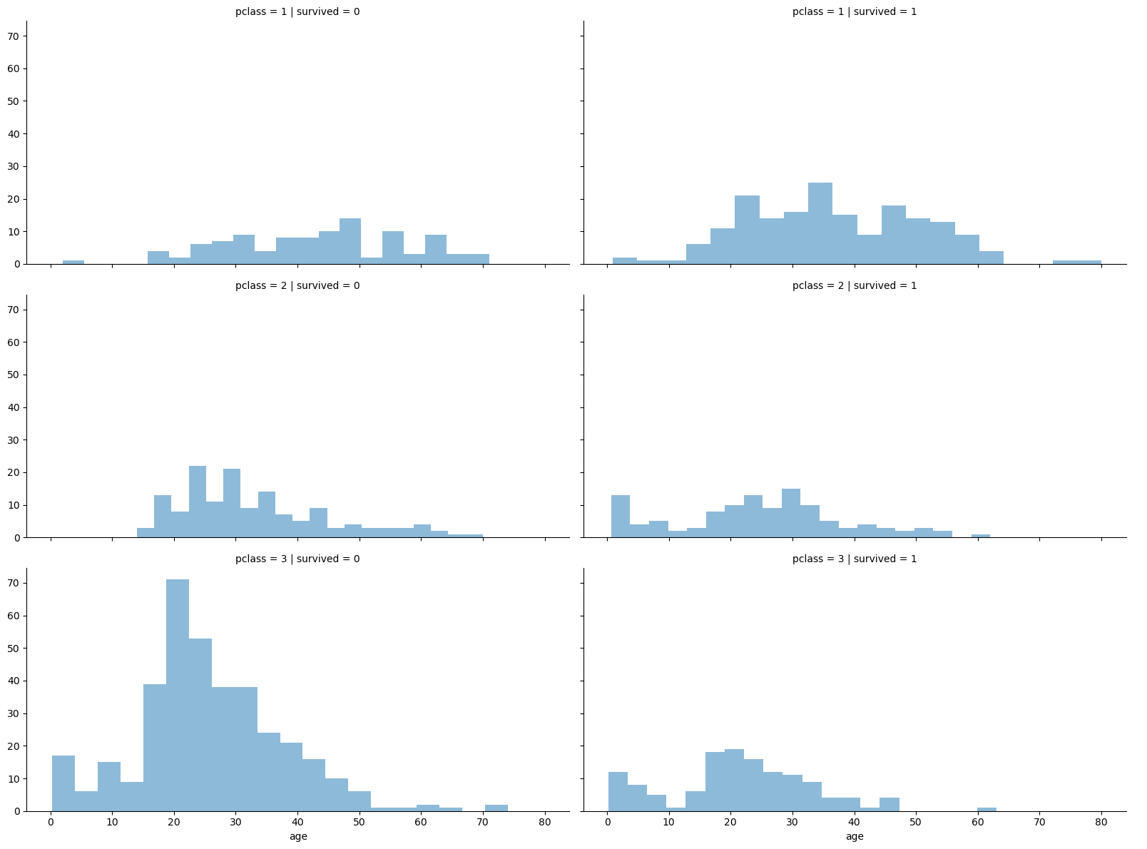

• 나이 5단계로 정리

titanic['age_cat'] = pd.cut(titanic['age'], bins=[0, 7, 15, 30, 60, 100],
                            include_lowest=True,
                            labels=['baby', 'teen', 'young', 'adult', 'old'])    
titanic.head()        

plt.figure(figsize=(12, 4))
plt.subplot(131) # 1행 3열 중 첫 번째
sns.barplot(x='pclass', y='survived', data=titanic)

plt.subplot(132)
sns.barplot(x='age_cat', y='survived', data=titanic)

plt.subplot(133)
sns.barplot(x='sex', y='survived', data=titanic)

plt.show()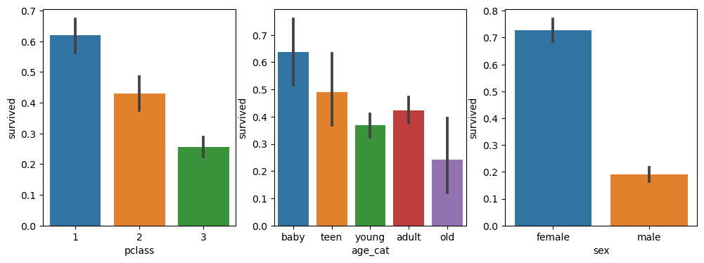

--> 어리고 여성이고 1등실일수록 생존률 높음

• 줄: 신뢰구간

fig, axes = plt.subplots(nrows=1, ncols=2, figsize=(14, 6))

women = titanic[titanic['sex']=='female']
men = titanic[titanic['sex']=='male']

ax = sns.distplot(women[women['survived']==1]['age'], bins=20, label='survived', ax=axes[0], kde=False)
ax = sns.distplot(women[women['survived']==0]['age'], bins=40, label='not survived', ax=axes[0], kde=False)
ax.legend(); ax.set_title('Female')

ax = sns.distplot(men[men['survived']==1]['age'], bins=18, label='survived', ax=axes[1], kde=False)
ax = sns.distplot(men[men['survived']==0]['age'], bins=40, label='not survived', ax=axes[1], kde=False)
ax.legend(); ax.set_title('Male')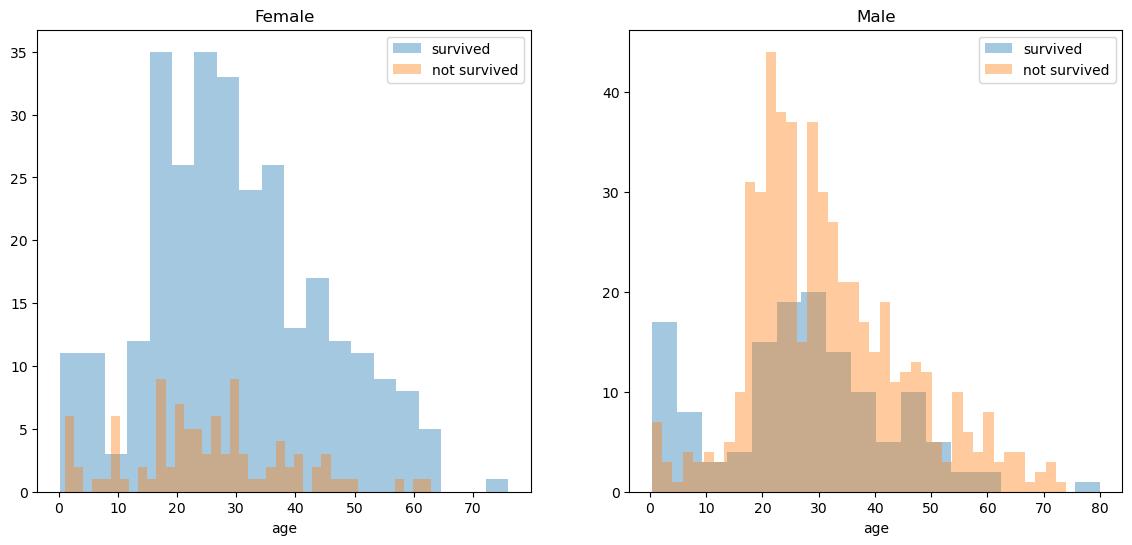

import re


title = []
for idx, dataset in titanic.iterrows():
    tmp = dataset['name']
    title.append(re.search('\,\s\w+(\s\w+)?\.', tmp).group()[2:-1])
    print(re.search('\,\s\w+(\s\w+)?\.', tmp).group())

titanic['title'] = title
titanic.head()

pd.crosstab(titanic['title'], titanic['sex'])

titanic['title'] = titanic['title'].replace('Mlle', 'Miss')
titanic['title'] = titanic['title'].replace('Ms', 'Miss')
titanic['title'] = titanic['title'].replace('Mme', 'Mrs')

Rare_f = ['Dona', 'Lady', 'the Countess']
Rare_m = ['Capt', 'Col', 'Don', 'Major', 'Rev', 'Sir', 'Dr', 'Master', 'Jonkheer']

for each in Rare_f:
    titanic['title'] = titanic['title'].replace(each, 'Rare_f')

for each in Rare_m:
    titanic['title'] = titanic['title'].replace(each, 'Rare_m')

titanic[['title', 'survived']].groupby(['title'], as_index=False).mean()

머신러닝을 이용한 생존자 예측

• LabelEncoder

from sklearn.preprocessing import LabelEncoder

le = LabelEncoder()
le.fit(titanic['sex'])

• 성별 -> 숫자

le.classes_

--> array(['female', 'male'], dtype=object)

titanic['gender'] = le.transform(titanic['sex'])
titanic.head()

---

• 결측치 포기

titanic = titanic[titanic['age'].notnull()]
titanic = titanic[titanic['fare'].notnull()]
titanic.info()

from sklearn.model_selection import train_test_split

X = titanic[['pclass', 'age', 'sibsp', 'parch', 'fare', 'gender']]
y = titanic['survived']

X_train, X_test, y_train, y_test = train_test_split(X, y, test_size=0.8, random_state=13)

from sklearn.tree import DecisionTreeClassifier
from sklearn.metrics import accuracy_score

dt = DecisionTreeClassifier(max_depth=4, random_state=13)
dt.fit(X_train, y_train)

pred = dt.predict(X_test)
print(accuracy_score(y_test, pred))

--> 0.7655502392344498

---

# [['pclass', 'age', 'sibsp', 'parch', 'fare', 'gender']]

import numpy as np

dicaprio = np.array([[3, 18, 0, 0, 5, 1]])  # 디카프리오 data 특정하기
print('Dicaprio: ', dt.predict_proba(dicaprio)[0, 1])

--> Dicaprio: 0.22950819672131148
생존률 23 %

winslet = np.array([[1, 16, 1, 1, 100, 0]])
print('Winslet: ', dt.predict_proba(winslet)[0, 1])

--> Winslet: 1.0
생존률 100 %