[CS231n] Assignment1 Q1: K-NN Classifier

드디어 CS231n 과제가 끝이 보이기 시작했다! 사실 assignment 하나 끝낼 때마다 복습 겸 기록해두려고 했는데 assignment3까지 모두 끝내는 것에 마음을 계속 쓰다보니 이제서야 기록을 하게 되었다... ㅎㅎ;;

아래는 공식 과제 링크
스탠포드 CS231n 공식 홈페이지의 과제 링크

아래는 내 풀이 링크
https://github.com/syhwang1231/cs231n

---

# Load the raw CIFAR-10 data.
cifar10_dir = 'cs231n/datasets/cifar-10-batches-py'

# Cleaning up variables to prevent loading data multiple times (which may cause memory issue)
try:
   del X_train, y_train
   del X_test, y_test
   print('Clear previously loaded data.')
except:
   pass

X_train, y_train, X_test, y_test = load_CIFAR10(cifar10_dir)

# As a sanity check, we print out the size of the training and test data.
print('Training data shape: ', X_train.shape)
print('Training labels shape: ', y_train.shape)
print('Test data shape: ', X_test.shape)
print('Test labels shape: ', y_test.shape)

먼저 classification에 쓸 CIFAR-10 데이터셋을 가져온다.

# output
Training data shape:  (50000, 32, 32, 3)
Training labels shape:  (50000,)
Test data shape:  (10000, 32, 32, 3)
Test labels shape:  (10000,)

# Subsample the data for more efficient code execution in this exercise
num_training = 5000
mask = list(range(num_training))
X_train = X_train[mask]
y_train = y_train[mask]

num_test = 500
mask = list(range(num_test))
X_test = X_test[mask]
y_test = y_test[mask]

# Reshape the image data into rows
X_train = np.reshape(X_train, (X_train.shape[0], -1))
X_test = np.reshape(X_test, (X_test.shape[0], -1))
print(X_train.shape, X_test.shape)

# output
(5000, 3072) (500, 3072)

training data set은 50000장, test data set은 10000장이므로 여기서 subsampling을 통해 training은 5000장, test는 500장으로 줄인다.
그 다음, 3*32*32 인 각 이미지를 1 row로 flatten한다. 3*32*32 = 3072이므로, 결과적으로 training의 shape은 50000*3072, test의 shape은 500*3072가 된다.

이제 K-NN 구현을 시작한다. K-NN classification은 총 2가지 스텝으로 이루어져있는 것을 기억하자.
1) 모든 test와 train examples 간의 distance 계산
2) distances가 주어졌을 때, 각 test example에 대해 k개의 가까운 example을 찾고 제일 많은 label로 선택

def compute_distances_two_loops(self, X):
  """
  Compute the distance between each test point in X and each training point
  in self.X_train using a nested loop over both the training data and the
  test data.

  Inputs:
  - X: A numpy array of shape (num_test, D) containing test data.

  Returns:
  - dists: A numpy array of shape (num_test, num_train) where dists[i, j]
  is the Euclidean distance between the ith test point and the jth training
  point.
  """
  num_test = X.shape[0]
  num_train = self.X_train.shape[0]
  dists = np.zeros((num_test, num_train))
  for i in range(num_test):
      for j in range(num_train):
          #####################################################################
          # TODO:                                                             #
          # Compute the l2 distance between the ith test point and the jth    #
          # training point, and store the result in dists[i, j]. You should   #
          # not use a loop over dimension, nor use np.linalg.norm().          #
          #####################################################################
          # *****START OF YOUR CODE (DO NOT DELETE/MODIFY THIS LINE)*****

          dists[i, j] = np.sqrt(np.sum((X[i] - self.X_train[j]) ** 2))

          # *****END OF YOUR CODE (DO NOT DELETE/MODIFY THIS LINE)*****
  return dists

첫번째로, 2개의 루프를 사용해서 거리를 계산하는 메소드를 구현한다. 모든 test, training example 쌍에 대해 for 루프를 돌면서 거리를 계산한다. 여기서는 L2 distance를 사용한다. X[i]는 i번째 test 데이터로, 1*3072 이고, self.X_train[j]는 j번째 training데이터로, 마찬가지로 1*3072이다. 3072개의 숫자들이므로 np.sum()을 통해 모두 더한 후 루트를 씌운다.

distance matrix 를 visualize 하면 위와 같이 된다.

Inline Question 1
Notice the structured patterns in the distance matrix, where some rows or columns are visibly brighter. (Note that with the default color scheme black indicates low distances while white indicates high distances.)
What in the data is the cause behind the distinctly bright rows?
What causes the columns?

• Your answer : each row = 하나의 테스트 데이터에 대한 모든 훈련 데이터의 거리들 → bright row 는 해당 test data가 모든 training data에 대해 많이 다름을 뜻함. 즉, 그 test data는 outlier이거나 노이즈일 수 있음.
  each column = 하나의 training data에 대한 모든 test data의 거리들 → bright column 은 해당 training data가 모든 test data에 대해 많이 다름을 뜻함. 즉, 그 training data는 outlier 이거나 대부분의 데이터가 갖지 않는 특이한 특징을 가졌을 수 있음.

def predict_labels(self, dists, k=1):
    """
    Given a matrix of distances between test points and training points,
    predict a label for each test point.

    Inputs:
    - dists: A numpy array of shape (num_test, num_train) where dists[i, j]
      gives the distance betwen the ith test point and the jth training point.

    Returns:
    - y: A numpy array of shape (num_test,) containing predicted labels for the
      test data, where y[i] is the predicted label for the test point X[i].
    """
    num_test = dists.shape[0]
    y_pred = np.zeros(num_test)
    for i in range(num_test):
        # A list of length k storing the labels of the k nearest neighbors to
        # the ith test point.
        closest_y = []
        #########################################################################
        # TODO:                                                                 #
        # Use the distance matrix to find the k nearest neighbors of the ith    #
        # testing point, and use self.y_train to find the labels of these       #
        # neighbors. Store these labels in closest_y.                           #
        # Hint: Look up the function numpy.argsort.                             #
        #########################################################################
        # *****START OF YOUR CODE (DO NOT DELETE/MODIFY THIS LINE)*****

        # 배열을 정렬한 인덱스 리스트, 처음 k개만 (제일 가까운 k개)
        closest_k_indices = np.argsort(dists[i])[:k]

        # 제일 가까운 k개의 인덱스에 해당하는 label 가져오기
        closest_y = self.y_train[closest_k_indices]

        # *****END OF YOUR CODE (DO NOT DELETE/MODIFY THIS LINE)*****
        #########################################################################
        # TODO:                                                                 #
        # Now that you have found the labels of the k nearest neighbors, you    #
        # need to find the most common label in the list closest_y of labels.   #
        # Store this label in y_pred[i]. Break ties by choosing the smaller     #
        # label.                                                                #
        #########################################################################
        # *****START OF YOUR CODE (DO NOT DELETE/MODIFY THIS LINE)*****

        # closest_y에서 중복되는 값은 모두 하나로만 하고 그것들의 개수도 같이 리턴
        unique_labels, counts = np.unique(closest_y, return_counts = True)

        # 개수가 제일 많은 것에 해당하는 unique_data 가져오기
        y_pred[i] = unique_labels[np.argmax(counts)]

        # *****END OF YOUR CODE (DO NOT DELETE/MODIFY THIS LINE)*****

    return y_pred

다음으로는, distance 행렬이 주어졌을 때 각 test point에 대해 label을 예측하는 predict_labels 메소드를 구현한다. 이때, 친절하게도 np.argsort()를 찾아보라고 힌트를 준다. np.argsort()는 배열을 정렬해 줄 수 있는 인덱스 배열을 리턴한다. 예를 들어, [13, 2, 9, 20] 이라는 배열이 있고, 여기에 argsort를 적용하면 output은 [1, 2, 0, 3] 이다.

그러면, np.argsort(dists[i])를 통해, i번째 test 데이터와 가까운 순서의 인덱스 배열을 얻고, [:k]로 슬라이싱하여 제일 가까운 k개의 인덱스 배열(closest_k_indices)을 구할 수 있게 된다! 구한 인덱스 배열을 통해 self.y_train에 접근해 제일 가까운 k개의 train 데이터의 정답 라벨을 구한다.

다음, k개의 label들 중 어떤 라벨이 제일 많은지 구한다. np.unique()를 통해 배열의 unique한 값들만 정렬해서 리턴해주는데, returns_counts=True로 설정해서 해당 값들의 개수도 같이 리턴하도록 한다. 이 배열을 np.argmax()에 넣어 제일 큰 값의 인덱스를 받는다. 그럼 이 값이 i번째 test 데이터의 예측된 y값이므로, y_pred[i]에 집어넣는다.

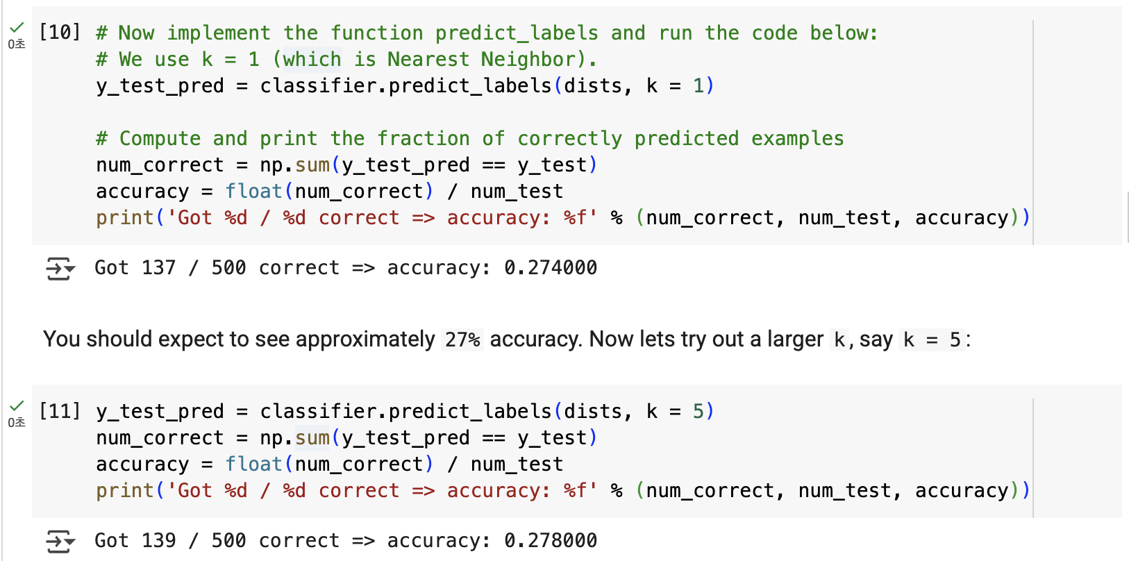
k=1, k=5 일 때 돌려보면 k=5일 때가 아주 약간 더 좋은 성능을 보이는 것을 확인할 수 있다.

Inline Question 2

We can also use other distance metrics such as L1 distance.
For pixel values $p_{ij}^{(k)}$ at location $(i,j)$ of some image $I_k$,

the mean $\mu$ across all pixels over all images is

And the pixel-wise mean $\mu_{ij}$ across all images is

The general standard deviation $\sigma$ and pixel-wise standard deviation $\sigma_{ij}$ is defined similarly.

Which of the following preprocessing steps will not change the performance of a Nearest Neighbor classifier that uses L1 distance? Select all that apply. To clarify, both training and test examples are preprocessed in the same way.

1. Subtracting the mean $\mu$ ($\tilde{p}_{ij}^{(k)}=p_{ij}^{(k)}-\mu$.)
2. Subtracting the per pixel mean $\mu_{ij}$ ($\tilde{p}_{ij}^{(k)}=p_{ij}^{(k)}-\mu_{ij}$.)
3. Subtracting the mean $\mu$ and dividing by the standard deviation $\sigma$.
4. Subtracting the pixel-wise mean $\mu_{ij}$ and dividing by the pixel-wise standard deviation $\sigma_{ij}$.
5. Rotating the coordinate axes of the data, which means rotating all the images by the same angle. Empty regions in the image caused by rotation are padded with a same pixel value and no interpolation is performed.

• $\color{blue}{\textit Your Answer:}$ 1, 2

• $\color{blue}{\textit Your Explanation:}$

  • 1. 모든 픽셀값을 같은 값만큼 shifting 해도 L1 distance는 같음.. = |x-y| = |(x-c)-(y-c)|
  • 2. 같은 위치의 픽셀에 대해서는 $\mu_{ij}$는 같음. 따라서 결국 {i,j}에서 $distance = |p_{ij}^{(k)}-p_{ij}^{(l)}| = |(p_{ij}^{(k)}-\mu_{ij})-(p_{ij}^{(l)}-\mu_{ij})|$

두번째 문제는 L1 distance를 쓰는 경우 K-NN의 성능에 영향을 미치지 않을 전처리를 고르는 문제이다.
처음 문제 풀 당시에는 1, 2로 선택했는데, 지금 다시 보니 3번도 어차피 같은 값만큼 shift하고 같은 값으로 나누는 것이므로 정답이 될 것 같다. 5번도... 마찬가지로 정답이 될 것 같네..... 흠냐뤼;;

def compute_distances_one_loop(self, X):
    """
    Compute the distance between each test point in X and each training point
    in self.X_train using a single loop over the test data.

    Input / Output: Same as compute_distances_two_loops
    """
    num_test = X.shape[0]  # 500 x 3072
    num_train = self.X_train.shape[0]  # 5000 x 3072
    dists = np.zeros((num_test, num_train))
    for i in range(num_test):
        #######################################################################
        # TODO:                                                               #
        # Compute the l2 distance between the ith test point and all training #
        # points, and store the result in dists[i, :].                        #
        # Do not use np.linalg.norm().                                        #
        #######################################################################
        # *****START OF YOUR CODE (DO NOT DELETE/MODIFY THIS LINE)*****

        # i번째 row의 테스트 데이터X와 전체 train data의 차이 계산
        diff = self.X_train - X[i, :]  # Shape: 5000 x 3072

        dists[i, :] = np.sqrt(np.sum(diff ** 2, axis = 1))

        # *****END OF YOUR CODE (DO NOT DELETE/MODIFY THIS LINE)*****
    return dists

이번엔 for 루프 한 번만으로 거리를 계산하는 메소드를 구현한다. 이제 numpy의 broadcasting 기능을 활용한다.
여기서 i는 test 데이터의 인덱스이다. X[i]의 Shape는 (3072,)이므로 self.X_train - X[i, :] 해주면 자동으로 broadcasting되어 self.X_train의 각 행에서 X[i, :]가 빼진다. 그런데 이 경우에는 X[i]라고 써도 되고 X[i, :]라고 써도 된다. 어쨌든 빼주면 diff는 i번째 row의 테스트 데이터와 전체 train data의 차이가 계산되어있고, 이 값을 제곱하고 모두 더해서 루트를 씌워주면 L2 distance가 계산되므로 dists[i, :]에 저장해준다.

def compute_distances_no_loops(self, X):
    """
    Compute the distance between each test point in X and each training point
    in self.X_train using no explicit loops.

    Input / Output: Same as compute_distances_two_loops
    """
    num_test = X.shape[0]  # X는 500 x 3072
    num_train = self.X_train.shape[0]  # X_train은 5000 x 3072
    dists = np.zeros((num_test, num_train))  # 500(r) x 5000(c)
    #########################################################################
    # TODO:                                                                 #
    # Compute the l2 distance between all test points and all training      #
    # points without using any explicit loops, and store the result in      #
    # dists.                                                                #
    #                                                                       #
    # You should implement this function using only basic array operations; #
    # in particular you should not use functions from scipy,                #
    # nor use np.linalg.norm().                                             #
    #                                                                       #
    # HINT: Try to formulate the l2 distance using matrix multiplication    #
    #       and two broadcast sums.                                         #
    #########################################################################
    # *****START OF YOUR CODE (DO NOT DELETE/MODIFY THIS LINE)*****

    # L2 계산 식 = \sigma (a-b)^2 = \sigma a^2 + \sigma b^2 - \sigma 2ab
    # 위처럼 각각 계산

    # X의 제곱들의 합 (axis=1이면 각 행을 열 방향으로 계산)
    # 얘는 keepdims=True로 해서 500x1로 열을 유지해야 밑에서 브로드캐스팅 가능함
    test_squared_sum = np.sum(X ** 2, axis = 1, keepdims=True) # 500 x 1

    # X_train의 제곱합
    train_squared_sum = np.sum(self.X_train ** 2, axis = 1) # 5000

    # 교차항 계산
    cross_term = -2 * np.dot(X, self.X_train.T)  # (500, 5000)

    # 최종 거리 계산 (L2 Norm)
    dists = np.sqrt(test_squared_sum + train_squared_sum + cross_term)  # Broadcasting 적용

    # *****END OF YOUR CODE (DO NOT DELETE/MODIFY THIS LINE)*****
    return dists

이제 마지막으로 루프 없이 L2 distance를 계산하는 메소드를 구현한다! 제공해주는 markdoc에서 어떤 메소드를 쓰지 말라고 해놨는데 어차피 난 저게 뭔 메소드인지도 모른다;; ㅎ;;
여기서 트릭은 L2 distance 계산 식을 전개하는 것이다. 그러면 X의 제곱들의 합, X_train의 제곱들의 합, X와 X_train의 곱을 각각 구하면 된다. 중요한 것은 keepdims=True로 해주어야 shape이 (500,)이 아니라 (500, 1)이 되고, 이렇게 차원을 유지해야 broadcasting이 가능하다는 것이다.
처음 두 항은 axis=1로 계산하는데, 이렇게 하면 열이 증가하는 방향으로 계산해서 행만 남는다. (찾아보는 것을 권장.. 해도해도 헷갈리는 개념이다) 결국 500*1이 된다.
axis=1로 해야 하는 이유는 추후에 교차항과 더할 때 broadcasting을 위해서인데, X의 Shape는 (500, 3072), X_train의 Shape는 (5000, 3072)이다. 따라서 이 두 행렬의 곱을 하려면 둘 중 하나가 transpose되어야 하고, 그 결과 곱셈의 결과는 (500, 5000)이 되어 3072라는 값이 날라간다. 따라서 axis=1로 해서 각각 500, 5000만 남게 하는 것이다.

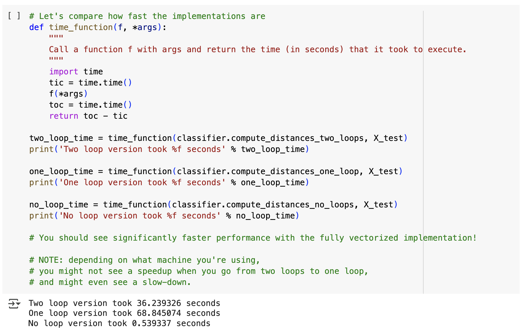
지금까지 구현한 메소드들의 실행 시간을 비교해보면, 루프를 쓰지 않은 메소드가 실행시간이 확연하게 짧은 것을 알 수 있다.

지금까지는 k라는 hyper parameter에 직접 값을 대입했는데, 이제부터는 cross-validation을 통해 k의 최적의 값을 찾아본다.

num_folds = 5
k_choices = [1, 3, 5, 8, 10, 12, 15, 20, 50, 100]

X_train_folds = []
y_train_folds = []
################################################################################
# TODO:                                                                        #
# Split up the training data into folds. After splitting, X_train_folds and    #
# y_train_folds should each be lists of length num_folds, where                #
# y_train_folds[i] is the label vector for the points in X_train_folds[i].     #
# Hint: Look up the numpy array_split function.                                #
################################################################################
# *****START OF YOUR CODE (DO NOT DELETE/MODIFY THIS LINE)*****

X_train_folds = np.array(np.array_split(X_train, num_folds))
y_train_folds = np.array(np.array_split(y_train, num_folds))

# *****END OF YOUR CODE (DO NOT DELETE/MODIFY THIS LINE)*****

# A dictionary holding the accuracies for different values of k that we find
# when running cross-validation. After running cross-validation,
# k_to_accuracies[k] should be a list of length num_folds giving the different
# accuracy values that we found when using that value of k.
k_to_accuracies = {}


################################################################################
# TODO:                                                                        #
# Perform k-fold cross validation to find the best value of k. For each        #
# possible value of k, run the k-nearest-neighbor algorithm num_folds times,   #
# where in each case you use all but one of the folds as training data and the #
# last fold as a validation set. Store the accuracies for all fold and all     #
# values of k in the k_to_accuracies dictionary.                               #
################################################################################
# *****START OF YOUR CODE (DO NOT DELETE/MODIFY THIS LINE)*****

k_nn_classifier = KNearestNeighbor()
for k in k_choices:
    k_to_accuracies[k] = []
    for i in range(num_folds):
        # validation fold (인덱스 i의 fold)
        X_val_fold = X_train_folds[i]
        y_val_fold = y_train_folds[i]

        # train fold (인덱스 i를 제외한 나머지 fold들)
        X_train_fold = np.concatenate([X_train_folds[j] for j in range(num_folds) if j != i], axis = 0)
        y_train_fold = np.concatenate([y_train_folds[j] for j in range(num_folds) if j != i], axis = 0)

        # k-nn 훈련
        k_nn_classifier.train(X_train_fold, y_train_fold)

        # k-nn predict
        y_pred = k_nn_classifier.predict(X_val_fold, k)

        # 정확도 계산 (둘이 같은지 t/f (1/0)여부)
        accuracy = np.mean(y_pred == y_val_fold)

        # k_to_accuracies에 저장
        k_to_accuracies[k].append(accuracy)

# *****END OF YOUR CODE (DO NOT DELETE/MODIFY THIS LINE)*****

# Print out the computed accuracies
for k in sorted(k_to_accuracies):
    for accuracy in k_to_accuracies[k]:
        print('k = %d, accuracy = %f' % (k, accuracy))

num_folds만큼 X_train과 y_train을 split해주고, k 값이 담긴 배열 k_choices의 루프를 돌면서, 해당 k값으로 실행했을 때의 accuracy를 저장한다. 두번째 for문에서는 cross-validation을 실행하면 된다.

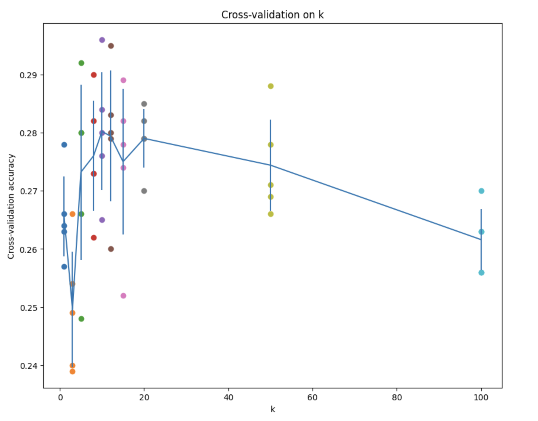
k값에 따른 정확도를 그래프로 표현해보면 위와 같다.

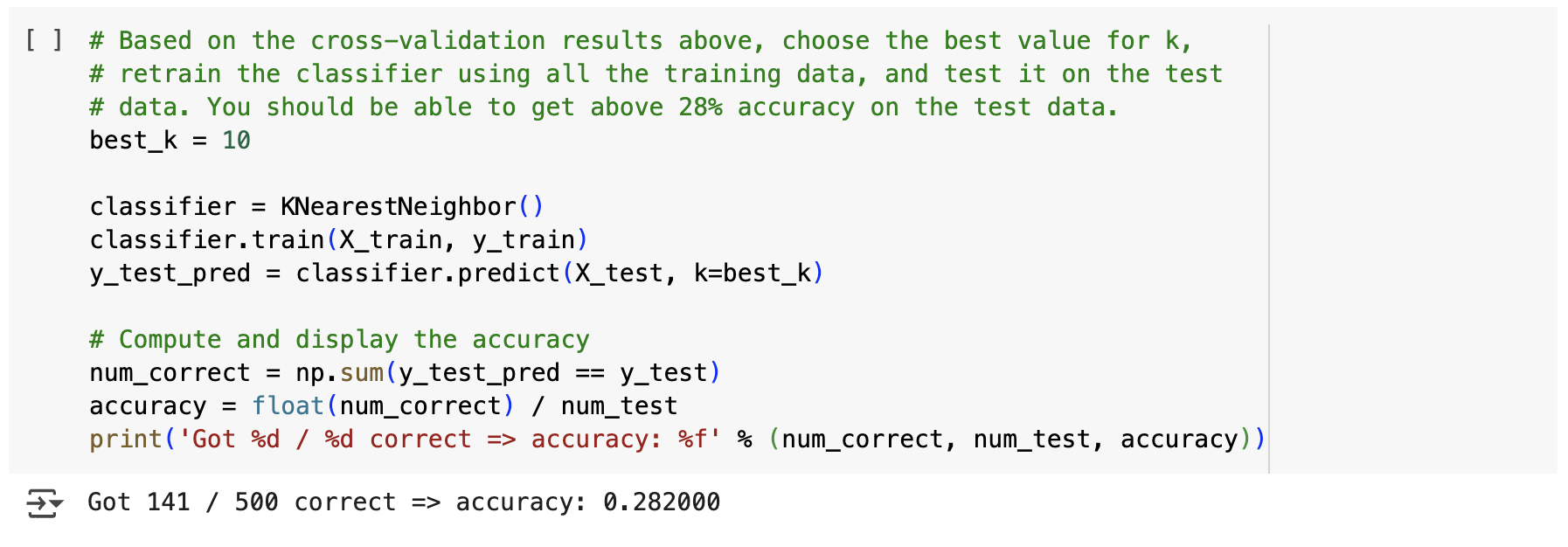
cross-validation의 결과를 토대로 최적의 k값을 선택해서 다시 train해보면, 위와 같은 정확도를 얻는다.

Inline Question 3

Which of the following statements about $k$-Nearest Neighbor ($k$-NN) are true in a classification setting, and for all $k$? Select all that apply.
1. The decision boundary of the k-NN classifier is linear.
2. The training error of a 1-NN will always be lower than or equal to that of 5-NN.
3. The test error of a 1-NN will always be lower than that of a 5-NN.
4. The time needed to classify a test example with the k-NN classifier grows with the size of the training set.
5. None of the above.

• $\color{blue}{\textit Your Answer:}$ 2, 4
• $\color{blue}{\textit Your Explanation:}$
  • 1 - k-NN은 예측 시에 거리를 기반으로 이웃을 찾아 다수결로 분류하기 때문에 linear가 아니라 더 복잡한 비선형 boundary를 가진다.
  • 2 - 1-NN은 자기 자신이 가장 가까운 이웃이기 때문에 항상 정확히 분류하므로 training error는 0이다.
  • 3 - 항상 그런 건 아님. 1-NN으로 train하면 오버피팅되므로 조금 더 일반화된 5-NN보다는 test error가 높겠지만, 항상 그런 것은 아니다.
  • 4 - training set가 더 많아질수록 test data와의 거리를 계산해야 하는 데이터가 많아지는 것이므로...

numpy를 사실 상 써본 적이 없는 수준이어서 맨땅에 헤딩이었던 과제였지만 또 그만큼 필요한 메소드를 먼저 써볼 수 있어서 좋았다! 과제도 정말 웰메이드였고 역시 스탠포드구나.. 싶었다 ㅎ