🔎 Stanford CS231n 강의를 듣고 기록용도로 정리하는 게시글입니다.

Inside ConvNets?

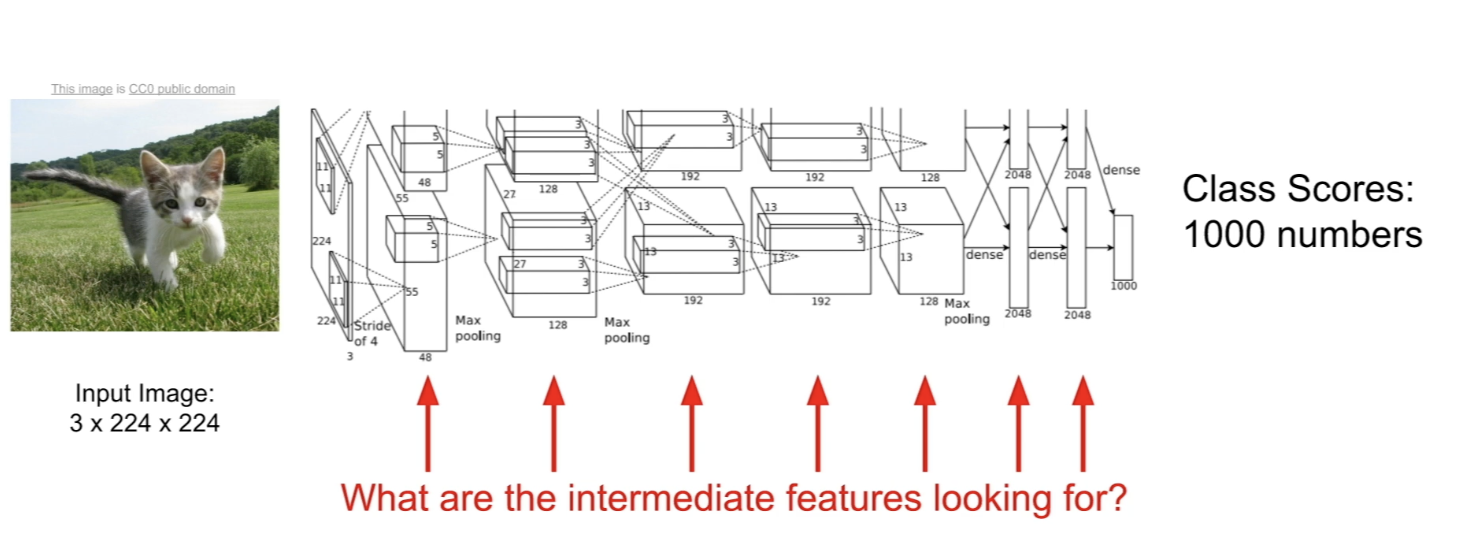
• so far, we've seen Convnets as a black box
  - input image of raw pixels come in on one side
  • goes through many layers of convolution, pooling, .. different sorts of transformation
  • end up with class scores or types of understandable interpretable output

First Layer: Visualize Filters

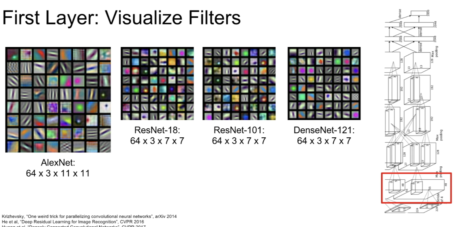
• in AlexNet,
  - convolutional filter of 3x11x11
  • filters slid over the input image, take inner products between chunk of the image and the weights of the convolutional filter
  • it's the output of the first convolutional layer
    - have 64 of these filters
• B/c we take direct inner product between the weights of the convolutional layer and the pixels of the image
  => can get some sense of what these filters are looking for, by visualizing the learned weights of these filters as images
  - lot of filters in AlexNet are looking for oriented edges, light and dark at various angles, positions, ...
  - connecting back to human visual system, which is known to detect things like oriented edges (Hugh and Wiesel) at the very early layers

????????
Q: Why does visualizing the weights of the filters tell you what the filter is looking for?
A: The intuition comes from template matching and inner products. Imagine you have a template vector and you compute a scalar output by taking an inner product between the template vector and some arbitrary piece of data. Then, the input which maximizes that activation under a norm constraint on the input is exactly when those 2 vectors match up. In that sense, whenever you take inner product, the thing that causes the inner product to excite maximally is a copy of the thing you're taking an inner product with.

Visualizing at higher layers

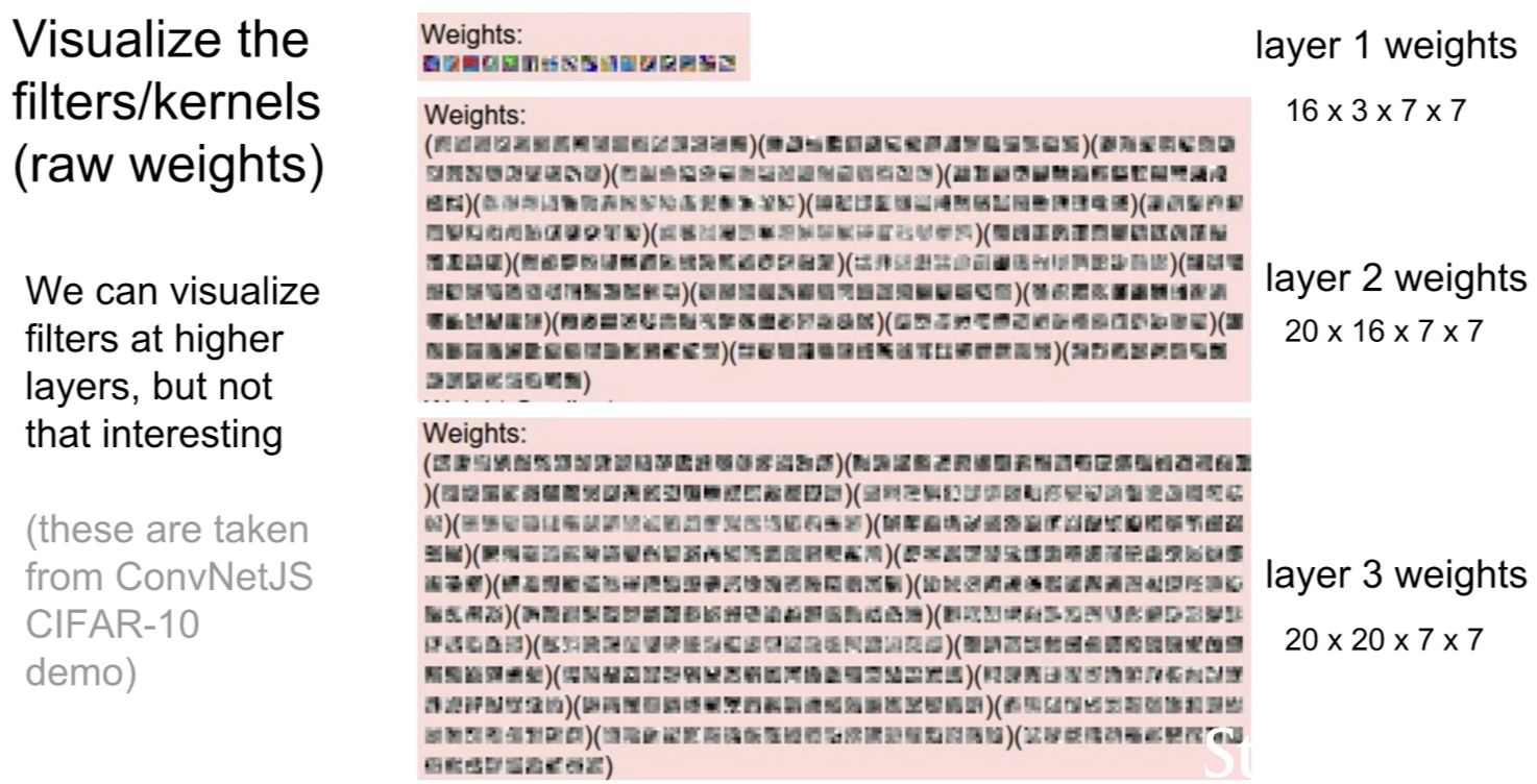
• we can visualize filters at higher layers, but less interpretable
• first layer is 7x7 convolution 16 filters
• after doing convolution, do some ReLU or other non-linearities
• second layer receives 16 channel input, and does 7x7 convolution with 20 filters
  - problem is that you can't really visualize these directly as images
  • 위에서는 20개 중 하나의 filter만 시각화한것 (16x7x7)
  • if we visualize the weights of those convolutional filters as images, you can see that there are some spatial structures here, but it doesn't give you a really good intuition of what they are looking at
    • b/c these filters are not connected directly to the input image
      • instead, these filters are connected to the "output" of the 1st layer
      • so, this is giving visualization of what type of activation pattern after the 1st convolution would cause the 2nd layer convolution to maximally activate
      • But this is not very interpretable, b/c we don't have a sense for what those first layer convolutions look like in terms of image pixels

Last layer

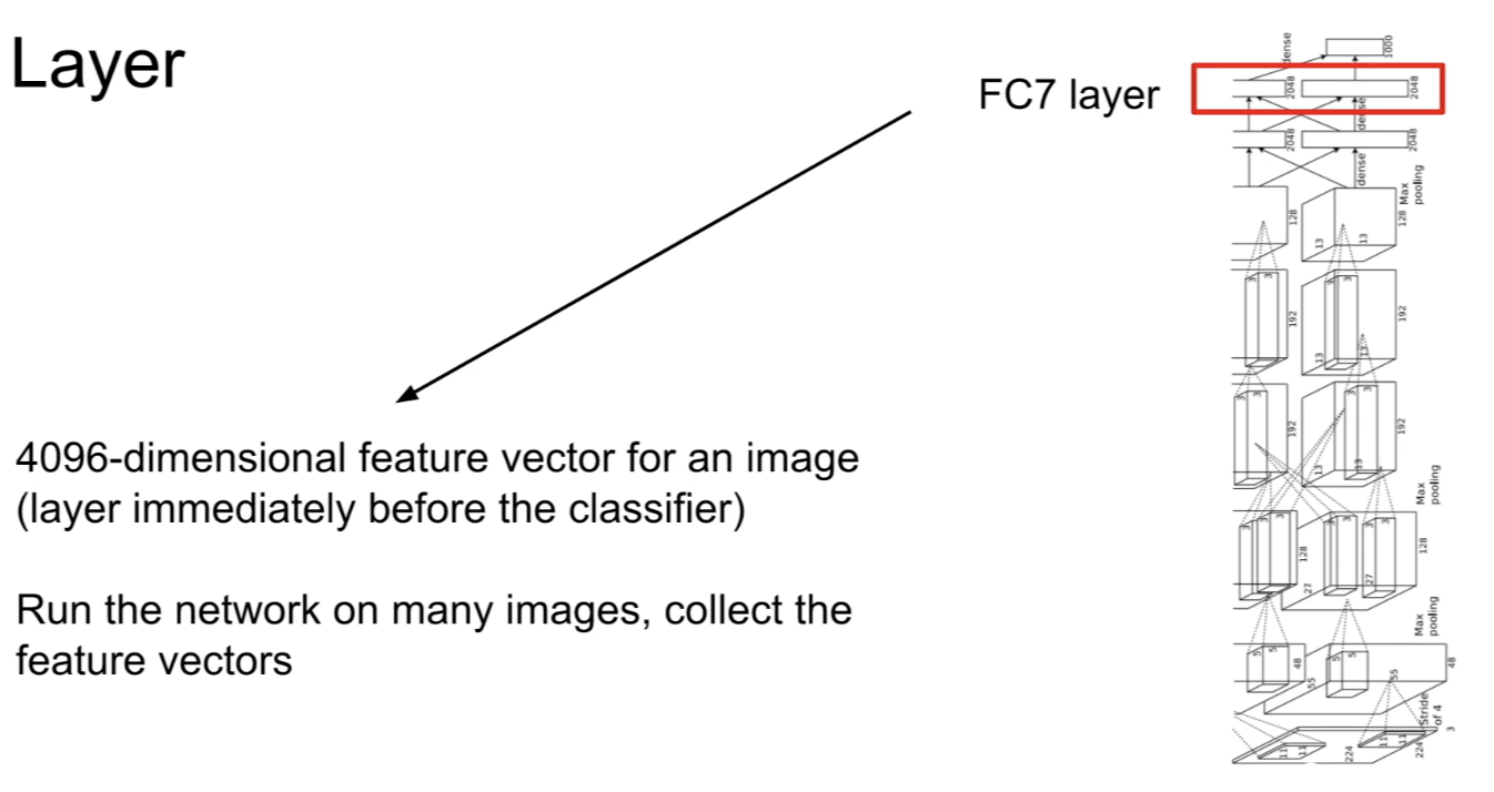
• maybe 1000 class scores that tells us what the predicted scores for each of the classes in the training data set are
• right before the last layer is FC layer
  - in AlexNet, we have 4096-dimensional feature representation of the image
  • then gets fed into the final layer to predict final class scores

Nearest Neighbor approach

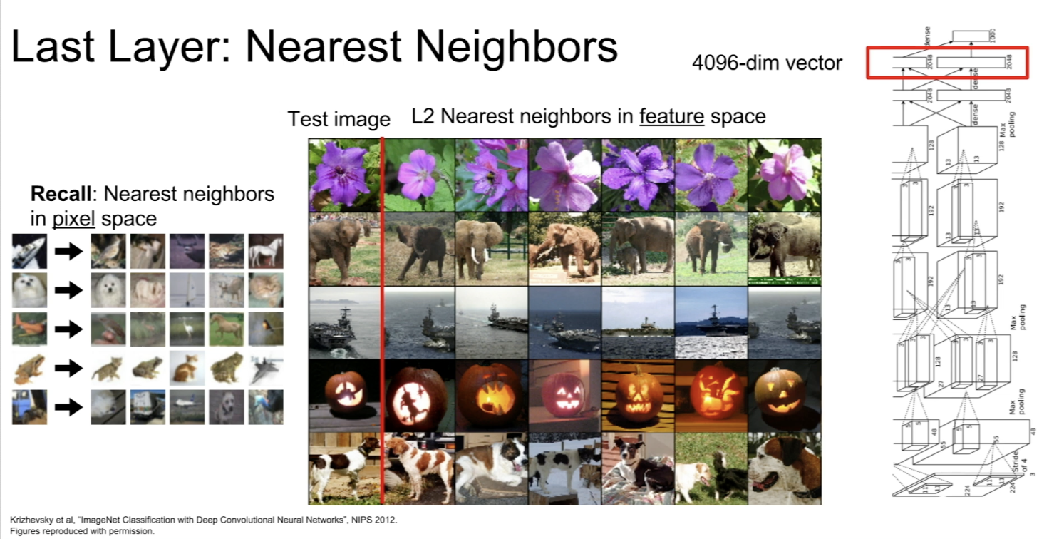
• rather than computing the nearest neighbors in pixel space,
• compute nearest neighbors in the 4096-dimensional feature space, which is computed by the ConvNet
  - 중간에 있는 그림이 이를 기준으로 NN을 계산한것
  • quite different from the pixel space NN, b/c pixels are often quite different between the image in it's nearest neighbors and feature space
• However, the semantic content of these images tend to be similar in this feature space
  - 2nd layer: query image is the elephant standing on the left side of the image with green grass behind him
  - 3rd NN - is an elephant standing on the right side of the image
  - this is interesting b/c the pixels between these 2 images are entirely different
  - however, in the feature space learned by the network, these 2 images end up being very close to each other = means that somehow this feature is capturing some of those semantic content of these images

Dimensionality Reduction

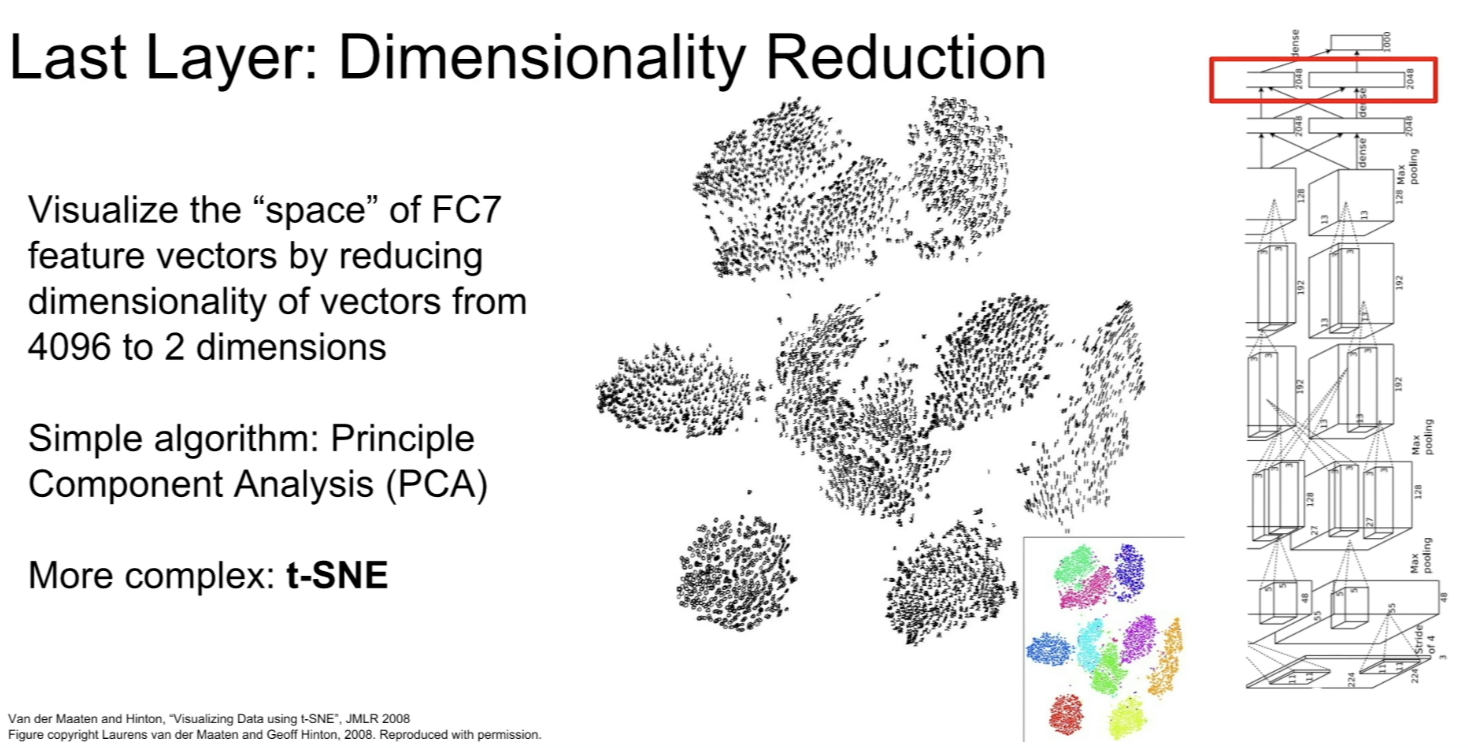
• a t-SNE dimensionality reduction on the MNIST data set
  - each image is a grayscale 28x28 image
  • compress it down to 2-D and visualize each of the MNIST digits in this compressed 2-D representation
• when you run t-SNE on raw pixels and MNIST -> natural clusters appear, which corresponds to the digits of the MNIST data set

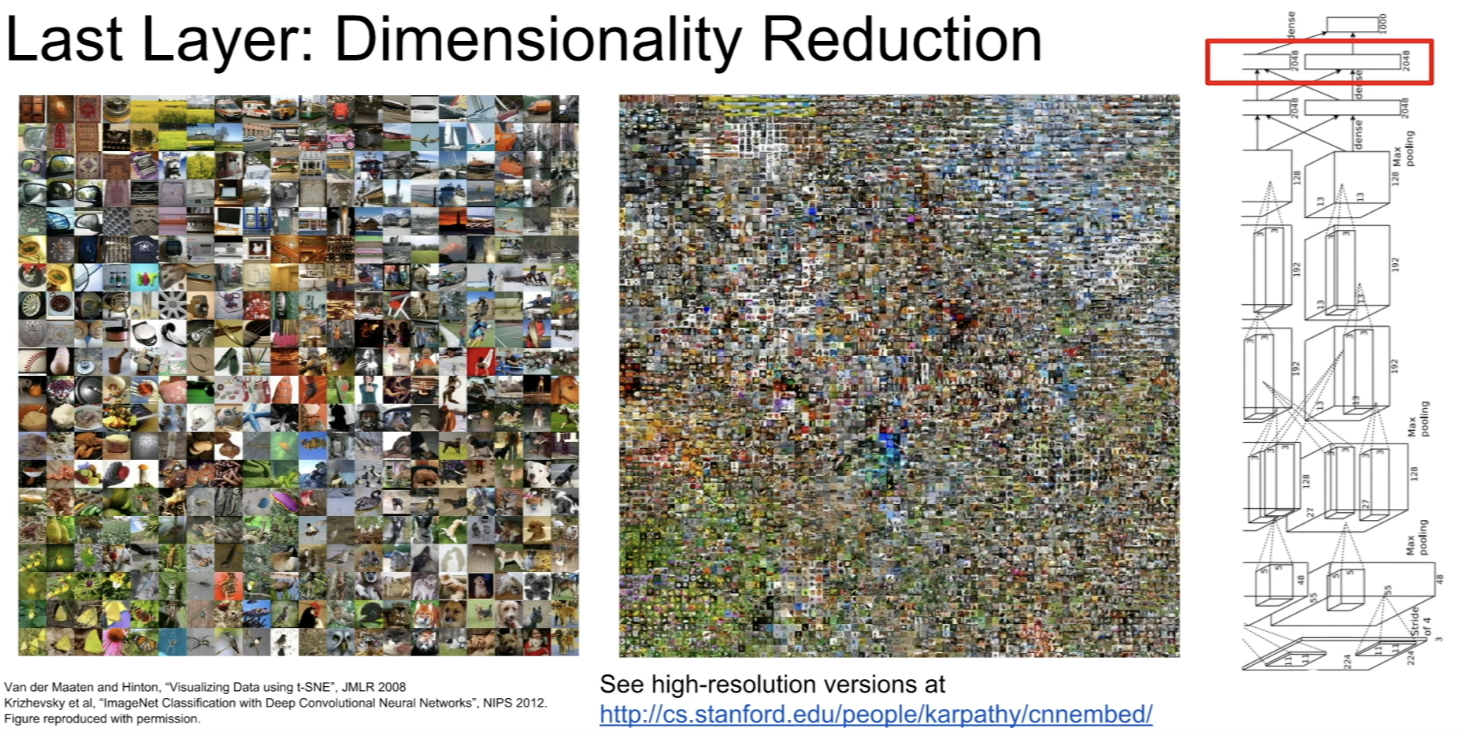
• now, we can apply t-SNE to the features from the last layer of the trained ImageNet classifier
  - take a large set of images, run them off the convnet, record that final 4096th-dimensional feature vector from the last layer for each of the images
  • apply t-SNE to compress 4096-dimensional feature space down into a 2-D feature space
  • layout a grid in that compressed 2-d feature space, and visualize what types of images appear at each location in the grid in this 2-d feature space
• there is discontinuous semantic notion in this feature space
  - one cluster on the bottom, of green things and different types of flowers
  - other cluster - different types of dog breeds
• basic idea: end up with 3 different information about the image; pixels of the image, 4096 dimensional vector, and use t-SNE to convert the 4096 dimensional vector into a 2D coordinate
  - so take the original pixels of the image, and place it at the 2-D coordinate corresponding to the dimensionality reduced version of the 4096th dimensional feature

Intermediate layers

Visualizing Activations

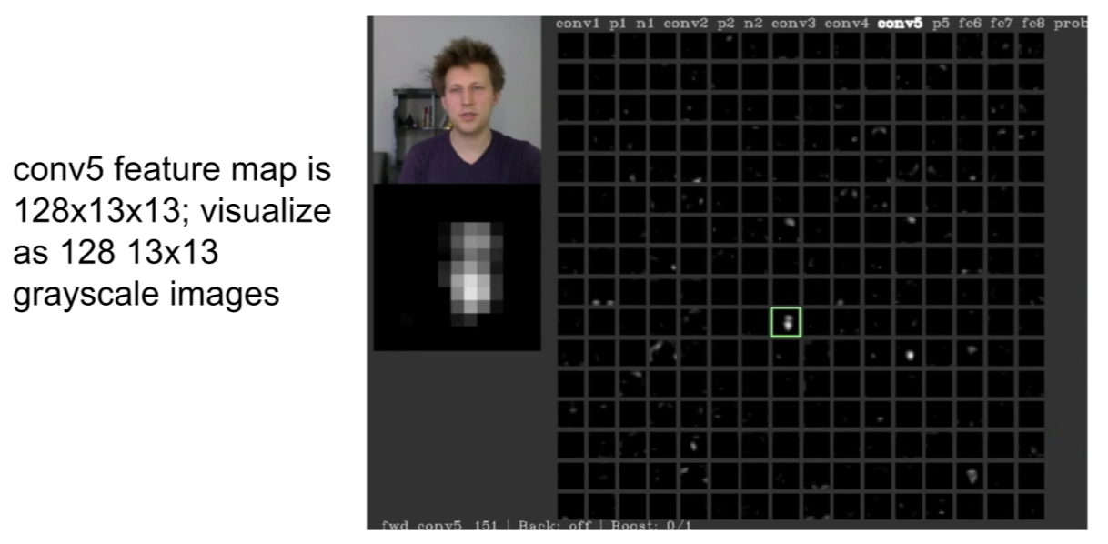
• visualize each of 13x13 element slices of the feature map as a grayscale image
  - gives some sense of what types of things in the input each of those features in that convolutional layer are looking for
• most of the intermediate features are noisy, and there's not much going on
• however, the highlighted intermediate feature seems activating on the portions of the feature map corresponding to the person's face
  - this suggests that this particular slice of the feature map of this layer of this particular network is maybe looking for human faces
  

Maximally Activating Patches

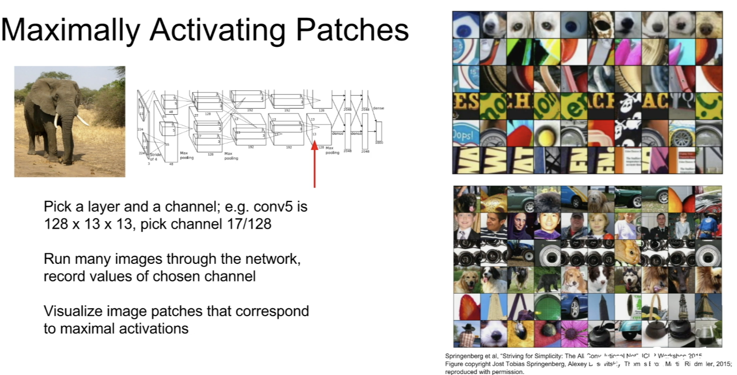
• Visualizing what types of patches from input images cause maximal activation in different neurons
• we've chosen 1 neuron from 1 layer of the network and the each row is the patch from some large data set of images that maximally activated this 1 neuron
  - gives some sense of what types of features these neurons might be looking for
  • (here, 'neuron' is 1 scalar value in that Conv5 activation map)

Occlusion Experiments

• occlusion (occlude: ~을 가리다, 막다):a process whereby something is hidden or obscured from prominence or view
  
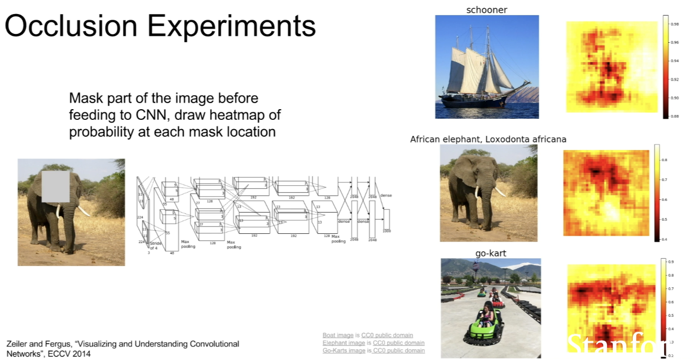
• want to figure out which parts of the input image cause the network to make it's classification decision
• take the input image and block out some region of that input image (=occluded image), and replace it with mean pixel value from the data set
• run that occluded image throughout the network, and record what the predicted probability of this occluded image is
  - 뭐에 대한 확률?
• then, slide the occluded patch over every position in the image and repeat the same process
• draw heat map showing what the predicted probability output from the network as a function of which part of the input image did we occlude was
• idea is that when we block out some part of the image and that causes the network score to change drastically, then probably that part of the image was really important for the classification decision

Saliency maps

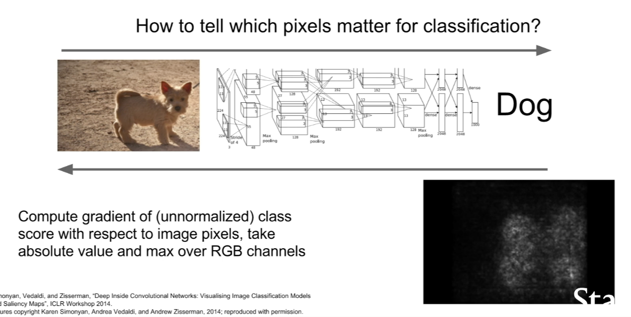
• given an input image (in this case, dog) and the predicted class label of dog, we want to know which pixels in the input image are important for classification
• computing the gradient of the predicted class score with respect to the pixels of the input image
  - this will directly tell us in first order approximation sense, for each pixel in the input image, if we wiggle that pixel a little bit, how much will the classification for the class change?
  • another way to get to the question of which pixels in the input matter for the classification
• when we compute a Saliency map for this dog, we see an outline of a dog in the image = these are pixels that the network is looking at for this image

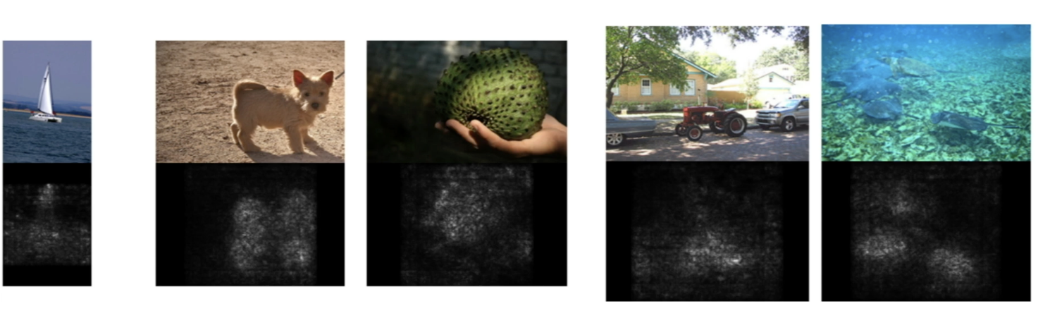
• when we repeat this for different iages, we get a sense that the network is looking at the right regions

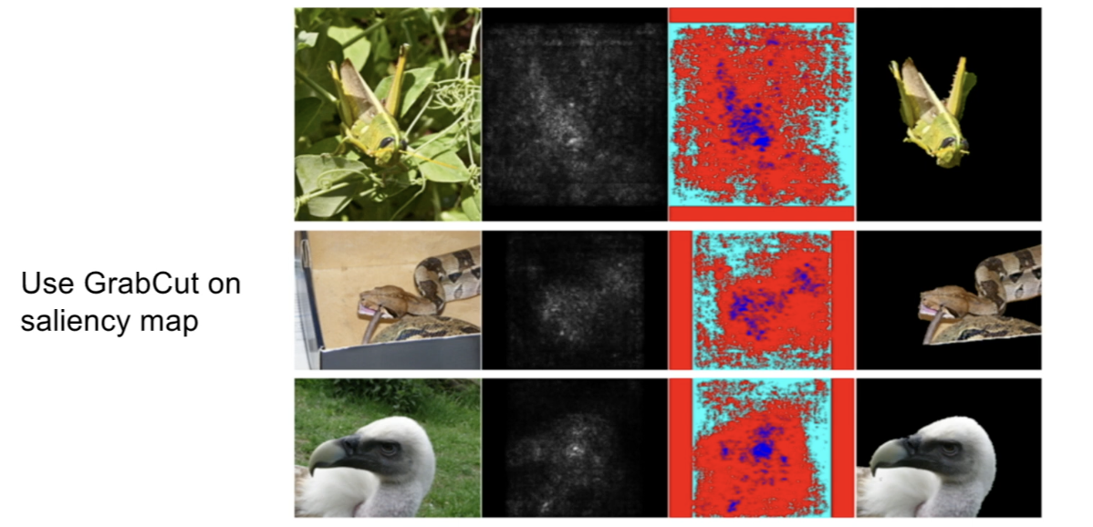
• we can actually use Saliency maps for segmentation, with Grabcut Segmentation Algorithm
  - in general, this works much worse than ones that had access to supervision in training time
  

Guided Backprop

• still want to answer the question of for one particular image, instead of looking at the class score, we want to pick some intermediate neuron and ask again, which parts of the image influence the score of that internal neuron in the network

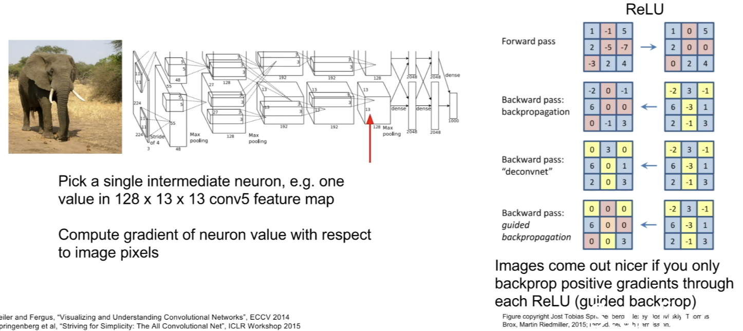
• change the way that you backprop through ReLU
  - only backprop positive gradients through ReLUs, and do not backprop negative gradients through ReLU
  • no longer computing true gradient
  • only keep track of positive influences throughout the entire network

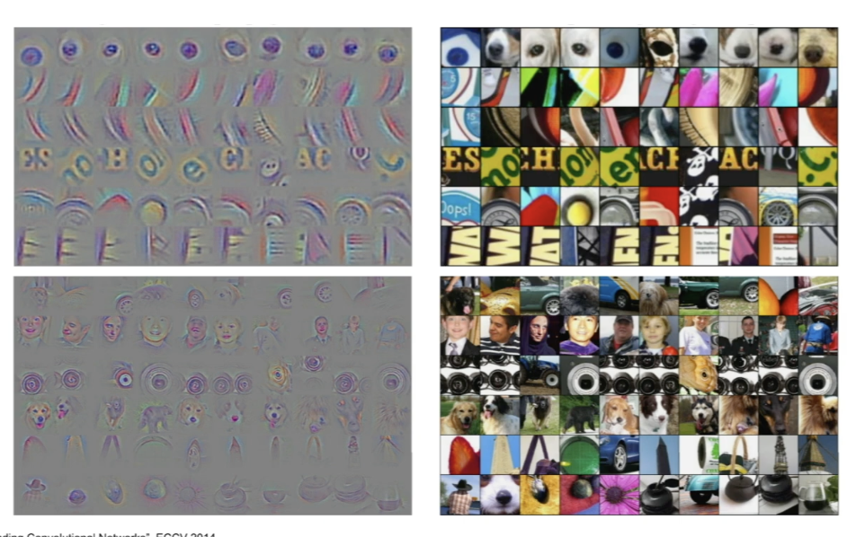
• when you do guided backprop, you tend to get much cleaner, nicer images that tell you which pixel of the input image influence that particular neuron

Gradient Ascent

• so far, there was a function of fixed input image, that tells us for a fixed input image, which pixel or part of that input image influence the value of the neuron
  - how about remove this reliance on some input image, and ask, in general what type of input would cause this neuron to activate
  => gradient ascent
  

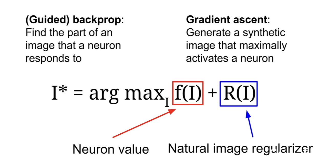
• fix the weight of the trained convolutional network and instead synthesize an image by performing Gradient Ascent on the pixels of the image to maximize the score of some intermedate neuron or of some class
• in Gradien Ascent, we no longer optimize over the weights of the network, but change pixels of some input image to cause this neuron or class score to be maximized
  - but in addition we need some regularization term (to prevent our generated image from overfitting to the peculiarities of the network, to enforce generated image to look relatively natural)

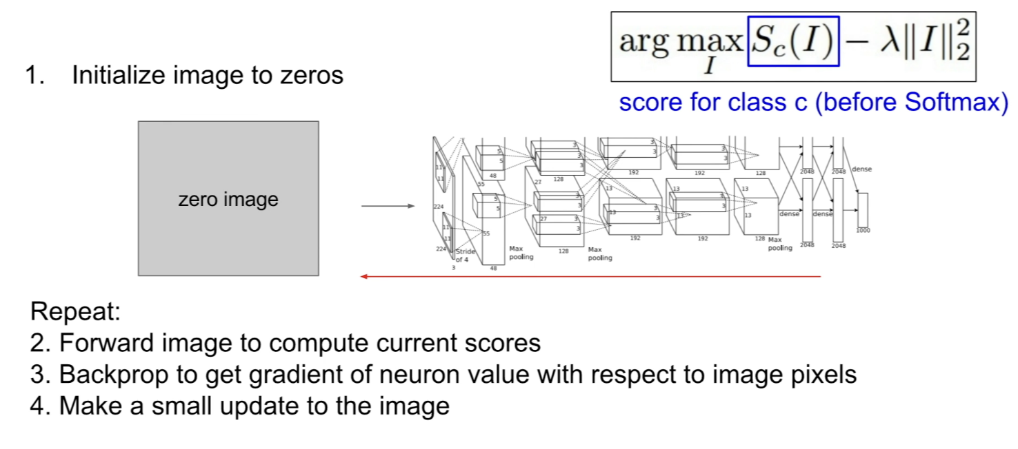
• repeat: forward your image through network and compute the score or neuron value that you're interested -> backprop to compute the gradient of that neuron score with respect to the pixels of the image -> make a small gradient descent or ascent update to the pixels of the image itself(to maximize the score)

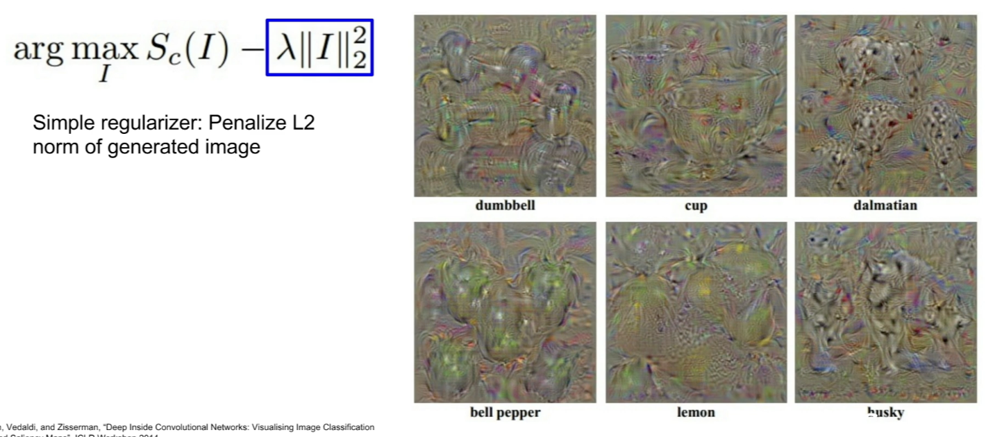
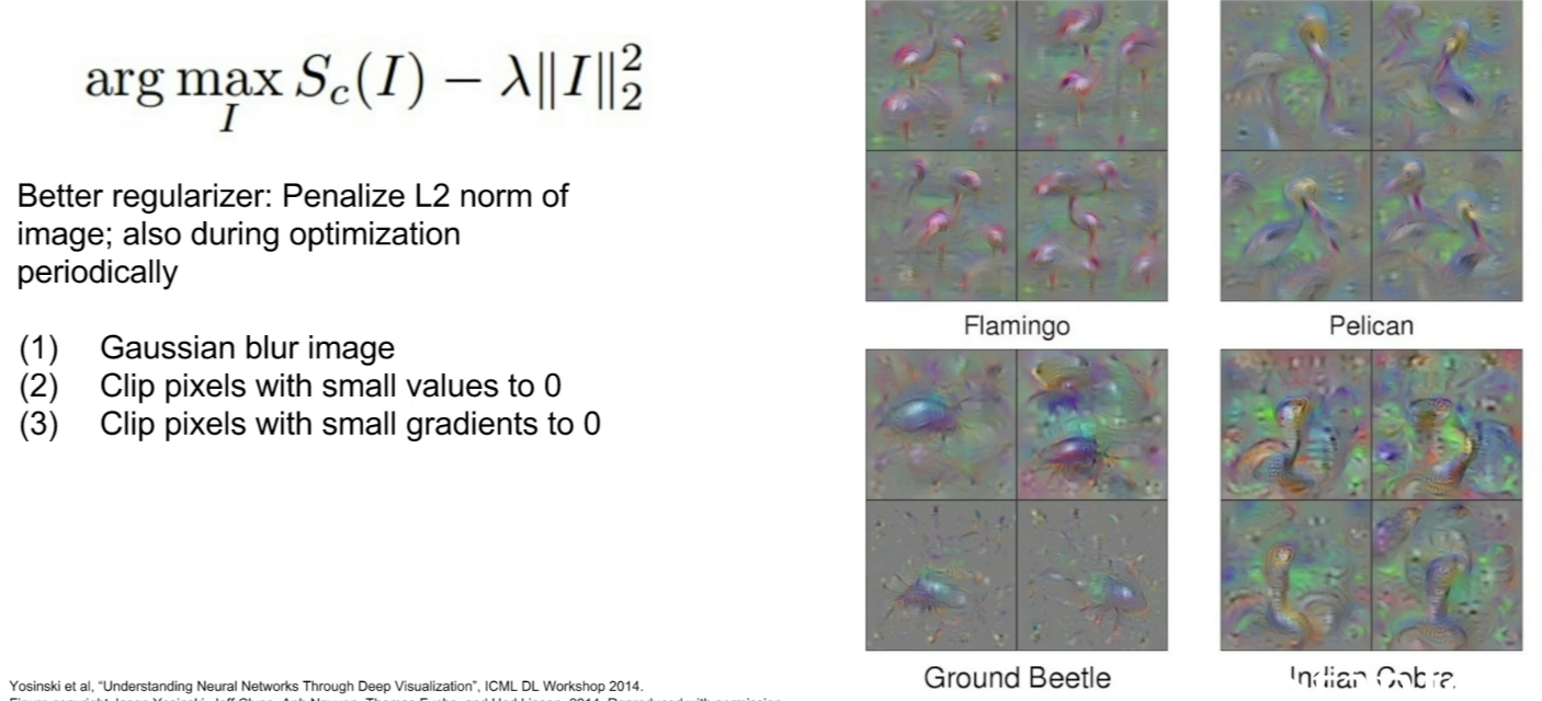
• here, they added an implicit regularizer

• in addition to L2 norm constraint, periodically during optimization, do some Gaussian blurring on the image, clip some small pixel values all the way to 0, or clip some of the pixel values of low gradients to 0

• this is kind of a projected Gradient descent algorithm, where we're periodically projecting our generated image onto some nicer set of images with some nicer properties

• we can perform this procedure not only for final class scores, but also for these intermediate neurons as well

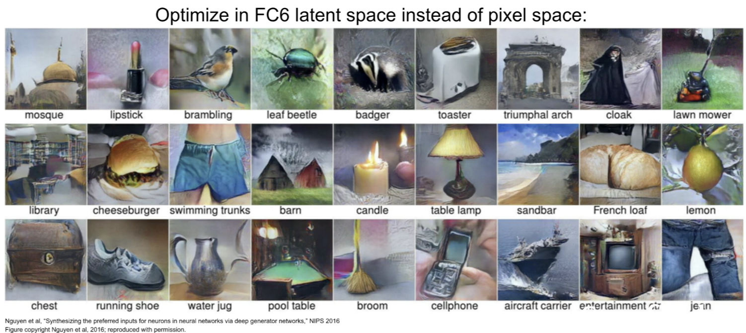
• rather than optimizing directly the pixels of the input image, optimize the FC6 representation of that image
• when you start adding additional priors(사전 확률) toward modeling natural images, you can end up generating realistic images that gave you some sense of what the network is looking for

Fooling Images / Adversarial Examples

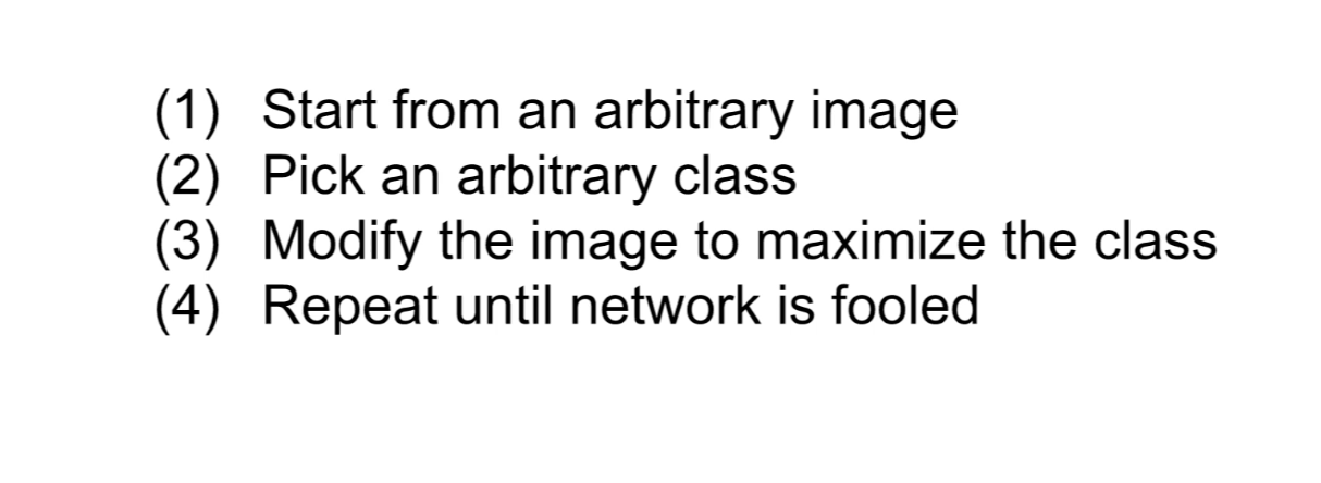
• idea of trying to synthesize images by using gradients on image pixels -> very powerful
• another thing that we can do with this = fooling images

• say that we take a picture of an elephant, and tell the network to change the image to maximize the score of Koala bear
  - so, we're trying to cause the network to classify this image of an elephant as a Koala bear
  - and what we hope for is that maybe that elephant will sort of start morphing(변하다) into a Koala bear...
  => but this is not what actually happens

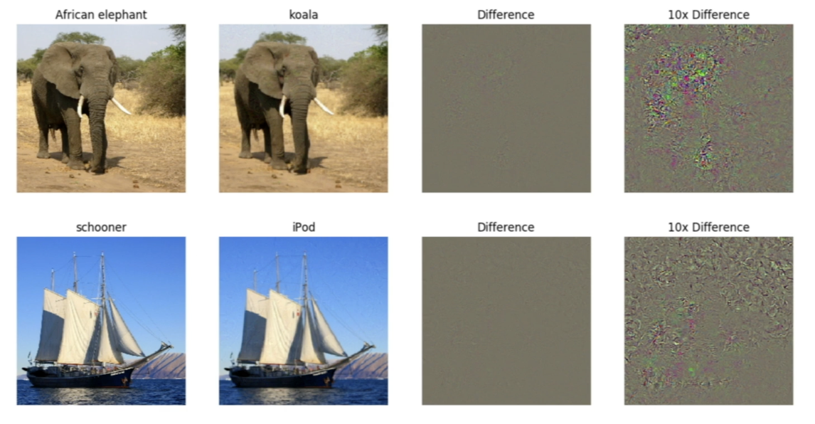
• second image on the right is actually classified as a Koala bear, but looks the same to us
• differences in pixels between two images are nothing
  - if you magnify differences, there's no iPod or Koala-like features, they're just random patterns of noise
  

Q: How does understading these intermediate neurons help our understanding of the final classification?
A: This field of trying to visualize intermediates is kind of in response to a common criticism of deep learning. The common criticism is that "you've got this big black box network, you trained it on gradient ascent, you get a good number, it's great, but we don't trust it because we don't understand as people, why it's making the decisions that it's making." A lot of these types of visualiation techniques are to say that these large complex models are still doing some intersting and interpretable things, not just totally going out in randomly classifying things.

DeepDream: Amplify existing features

• another cool thing that we can do with gradient based optimization of images

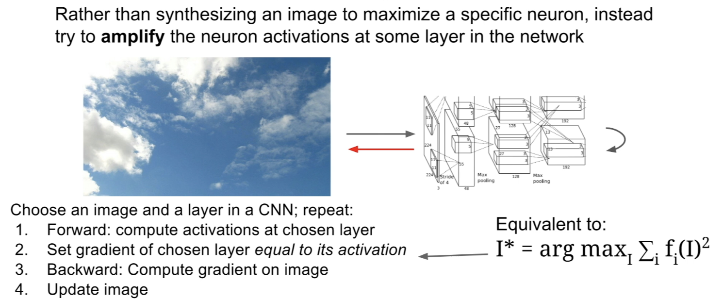
• take input, run it through ConvNet up to some layer, backprop and set the gradient of that layer equal to the activation value, then backprop back to the image, update the image and repeat
• this has the interpretation of trying to amplify existing features that were detected by the network in this image
  - b/c whatever features existed on that layer, we set the gradient equal to the feature and just tell the network to amplify whatever features it saw in that image
• you can also see this as trying to maximize the L2 norm of the features at that layer of the image

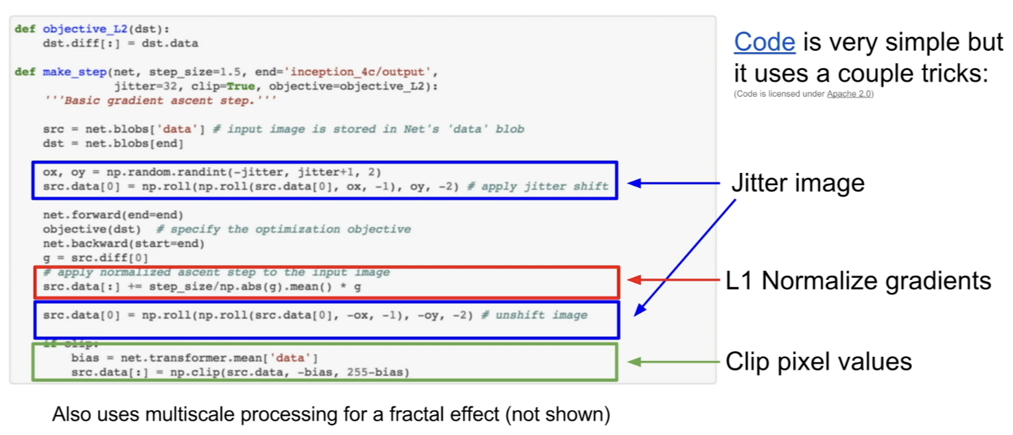
• couple of tricks
  - jitter the image before computing gradients - rather than running the exact image through the network, shift the image over by 2 pixels => kind of regularizer to encourage a little bit of extra special smoothness in the image
  - L1 normalization - kind of useful trick when generating images
  • clipping the pixel values once in a while - images should be between 0 to 255, so this is where we project onto the space of actual valid images

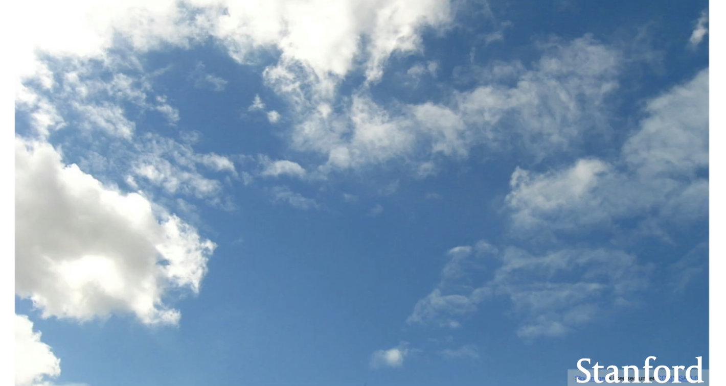
• when we start by an image of a sky

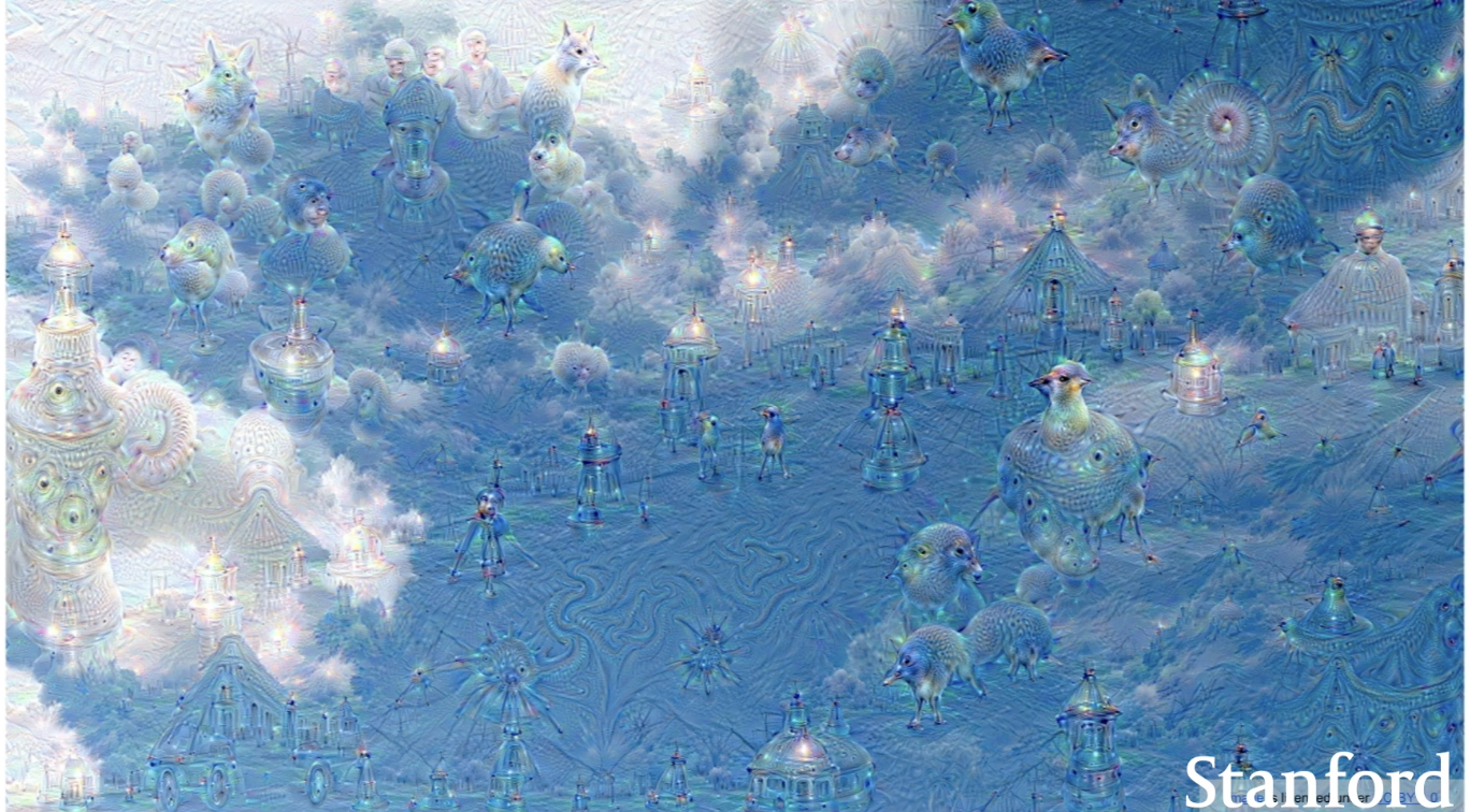
• we've taken tiny features on the sky and they get amplified through this process
  features????
• the fact that 'dogs' show up so much tells us something about the data that this network was trained on
  - this is a network that was trained for ImageNet classification, and ImageNet has thousands of categories, but 200 of those categories are dogs
  • not surprising in a sense that when you do these kinds of visualizations, the network ends up hallucinating a lot of dog like stuff in the image, often morphed with other types of animals

Feature Inversion

• gives us sense for what types of elements of the image are captured at different layers of the network
  
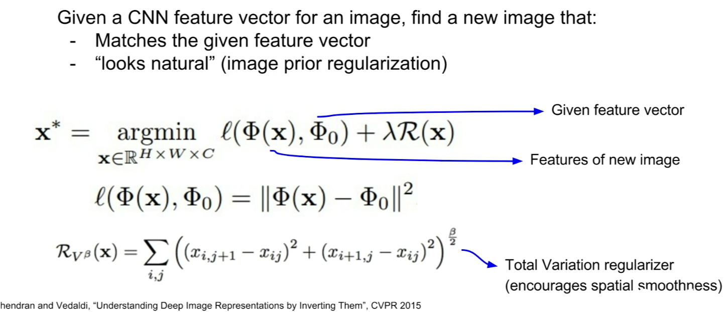
• run the input image through the network, record the feature value for one of those images, and try to reconstruct that image from its representation
• how the reconstructed image looks like will give us some sense for what type of information about the image was captured in that feature vector
  - we can do this with gradient ascent with some regularizer
  - minimize the distance between the cached feature vector and the computed features of the generated image
  • total variation regularizer - penalizing differences between adjacent pixels in the left to right and adjecent top to bottom (to encourage spatial smoothness)

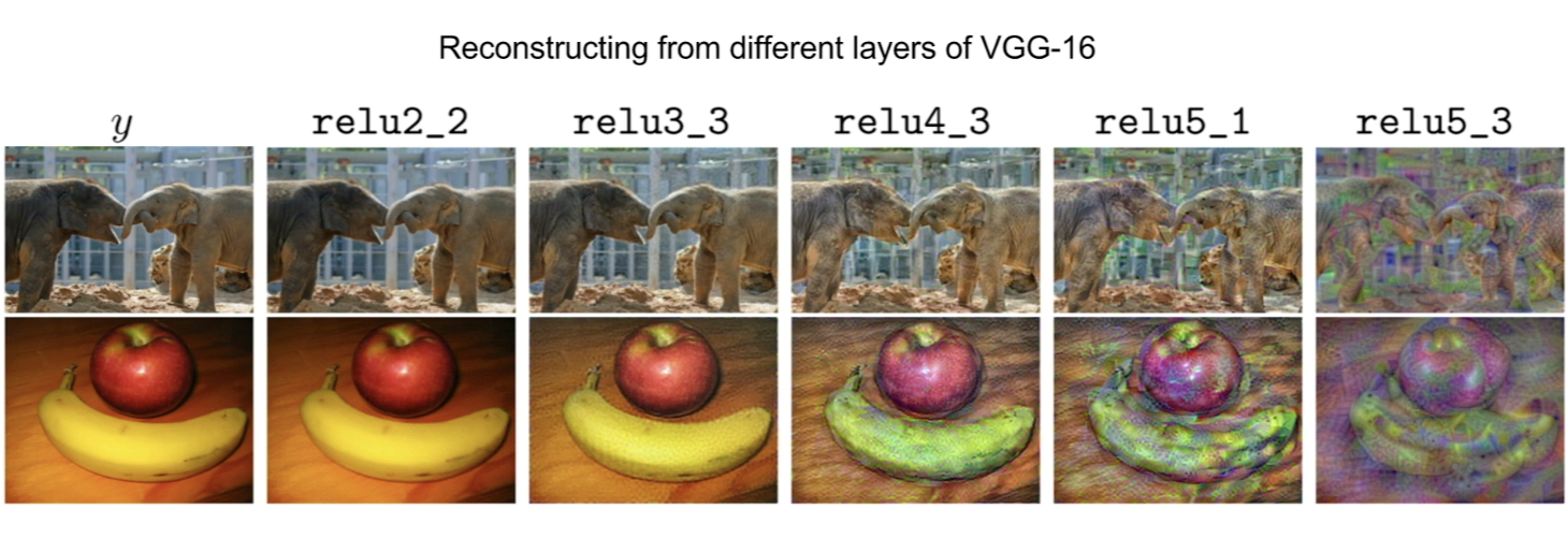
• if we try to reconstruct the image based on the ReLU2_2 features from VGG-16, we see that the image gets almost perfectly reconstructed
  - meaning that we're not throwing away much information about the raw pixels values at that layer
• as we move deeper in the network and try to reconstruct, now the reconstructed image keeps the general spatial structure of the image, but a lot of the low level details (ex. what exactly the pixel values are, what exactly the colors were ..) are lost
  - meaning that as we move up through the network, it throws away the low level details about the exact pixels of the image and try to keep around a more semantic information

Texture Synthesis

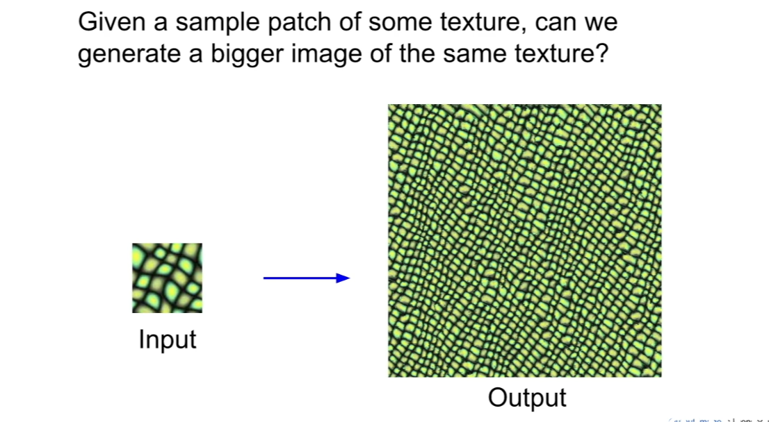
Nearest Neighbor Approach

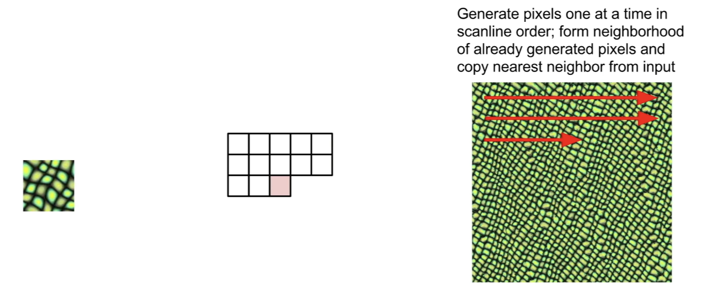
• march through generated image 1 pixel at a time in scan line order, and look at a neighborhood around the current pixel based on the pixels that we've already generated, compute a NN of that neighborhood in the patches of the input image and copy over 1 pixel from the input image
• no need to understand the detail
• idea is that you can do this without neural network
• works well for the simple textures, but as we move to more complex textures, these kinds of simple methods of copying pixels from the input patch directly tend not to work so well

Neural Texture Synthesis: Gram Matrix

• take the input texture and pass it through ConvNet, pull out conv features(CxHxW) at some layer of the network
• think of the conv features as an HxW spatial grid, with C dimensional feature vector at each point of the grid
  
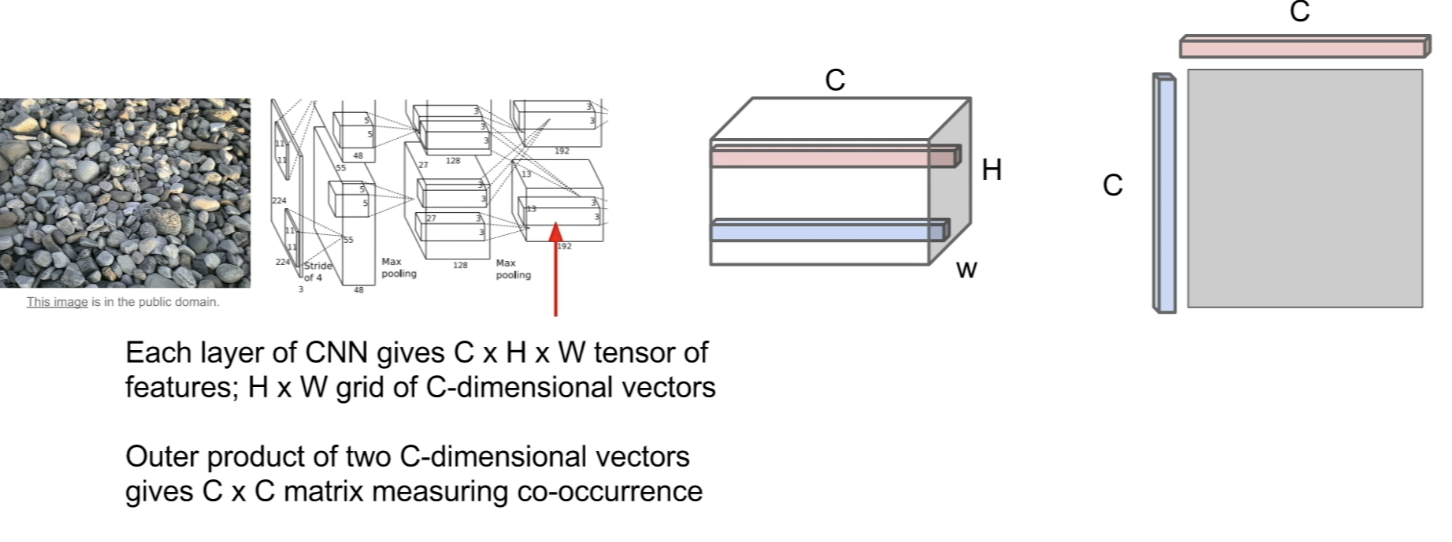
• use this activation map to compute a descriptor of the texture of this input image
  - pick out 2 of these feature columns in the input volume (each column being C-dimensional vector)
  • take the outer product between those 2 vectors that gives CxC matrix
  • this CxC matrix tells us something about the co-occurrence of the different features at those 2 points in the image
    • if element $IJ$ in the CxC matrix is large, it means both element $I$ and $J$ of those 2 input vectors were large...

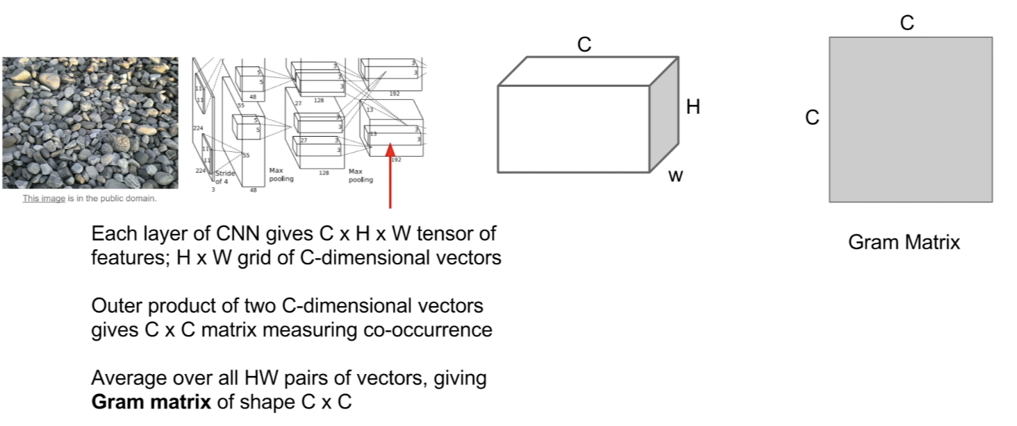
• repeat this procedure using all different pairs of feature vectors from all different points in HxW grid -> average them all out -> CxC gram matrix
  - this is then used as a descriptor to describe the texture of that input image
• Gram matrix has thrown away all spatial information that was in the feature volume
  - b/c we averaged all pairs of feature vectors at every point in the image
  • instead, it captures 2nd order co-occurrence statistics between features
• efficient to compute; reshape features from CxHxW to = C x HW then compute $G = FF^T$

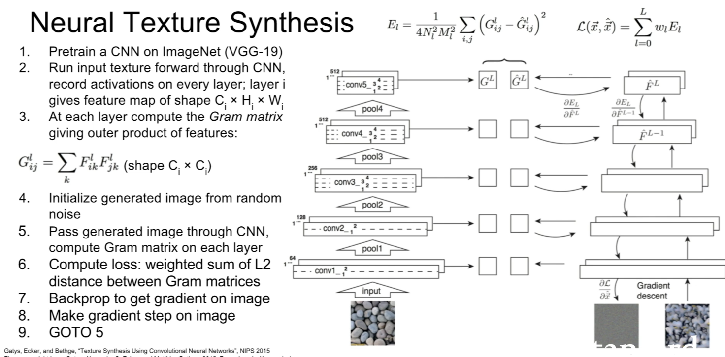
• now we can use a similar gradient ascent procedure to synthesize a new image that matches the texture of the original image

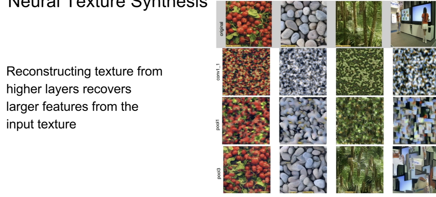
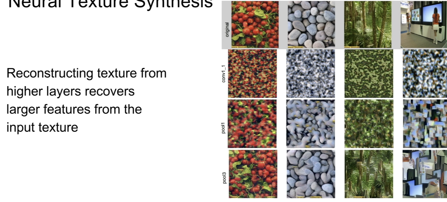
• if we use low layers
  - we get the splotches(얼룩) of the right colors but overall spatial structures doesn't get preserved so much
• as we move further in the network and compute gram matrix,
  - they tend to reconstruct larger patterns from the input image
  • quite different pixel wise from the actual input itself

Neural Texture Synthesis: Texture=Artwork

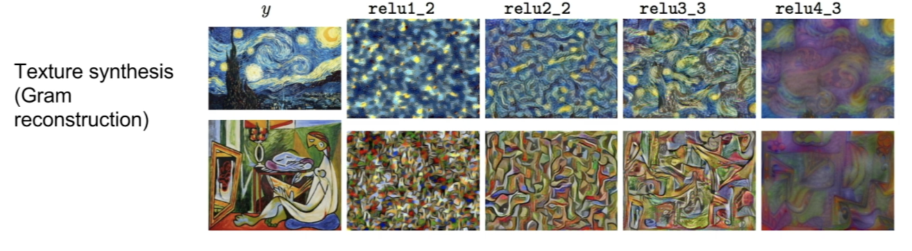
• do the same texture synthesis algorithm by maximizing gram matrices, but take artworks as our input texture... -> generated images tend to reconstruct pieces from those pieces of artwork

Neural Style Transfer

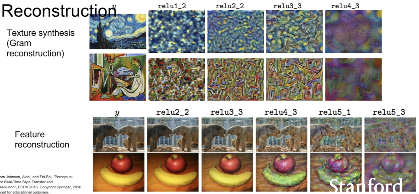
• combine texture synthesis by gram matrix matching and feature inversion by feature matching

• 2 input images; content image(guide what type of thing we want) + style image(general texture or style that we want the generated image to have)
• generate a new image by minimizing the feature reconstruction loss of the content image and the gram matrix loss of the style image

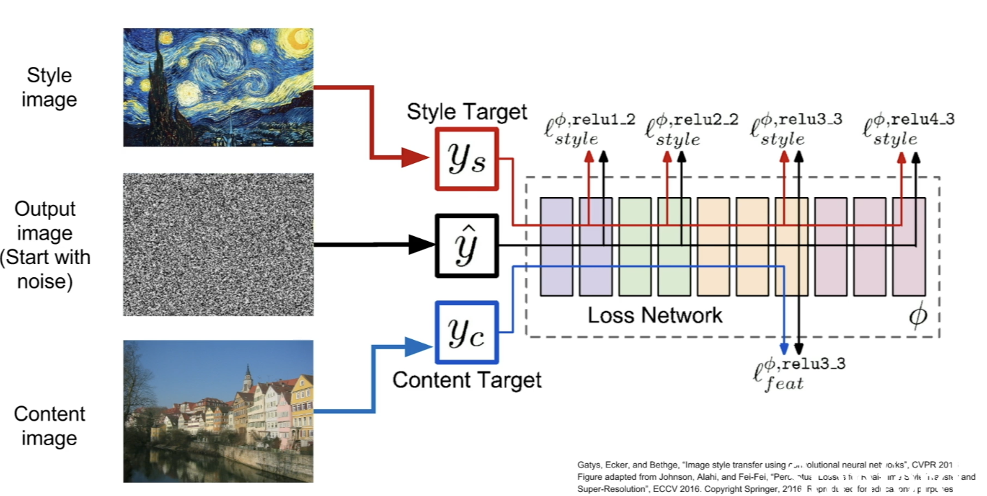
• pass input images into network to compute gram matrices and features
• initialize the output image with some random noise
• go forward, compute losses
• go backward, compute gradients on the image
• repeat this process over and over, doing gradient ascent on the pixels of your generated image

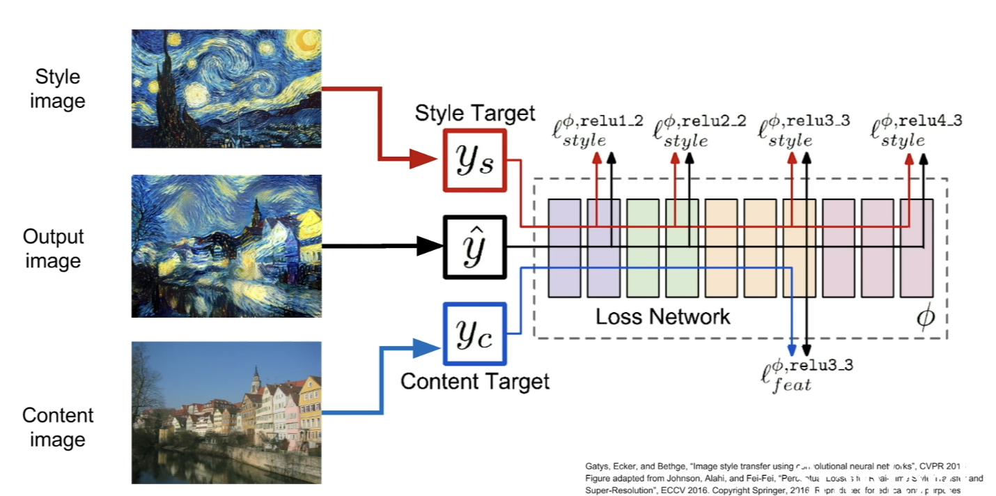
• after few 100 iterations generally, you get the output

• compared to DeepDream
  - give you more control over the generated image
  - in DeepDream, you can only pick different layers at the network
  - in StyleTransfer, you get more control over what you want the result to look like (picking different style iamges with same content image)

Changing Hyperparameters

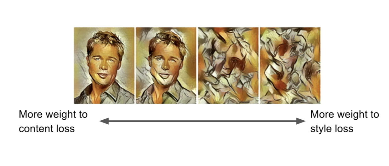
• trading off the weighting between feature reconstruction loss of the content image and gram matrix reconstruction loss of the style image
  - can get control about how much we want to match the content versus style
  

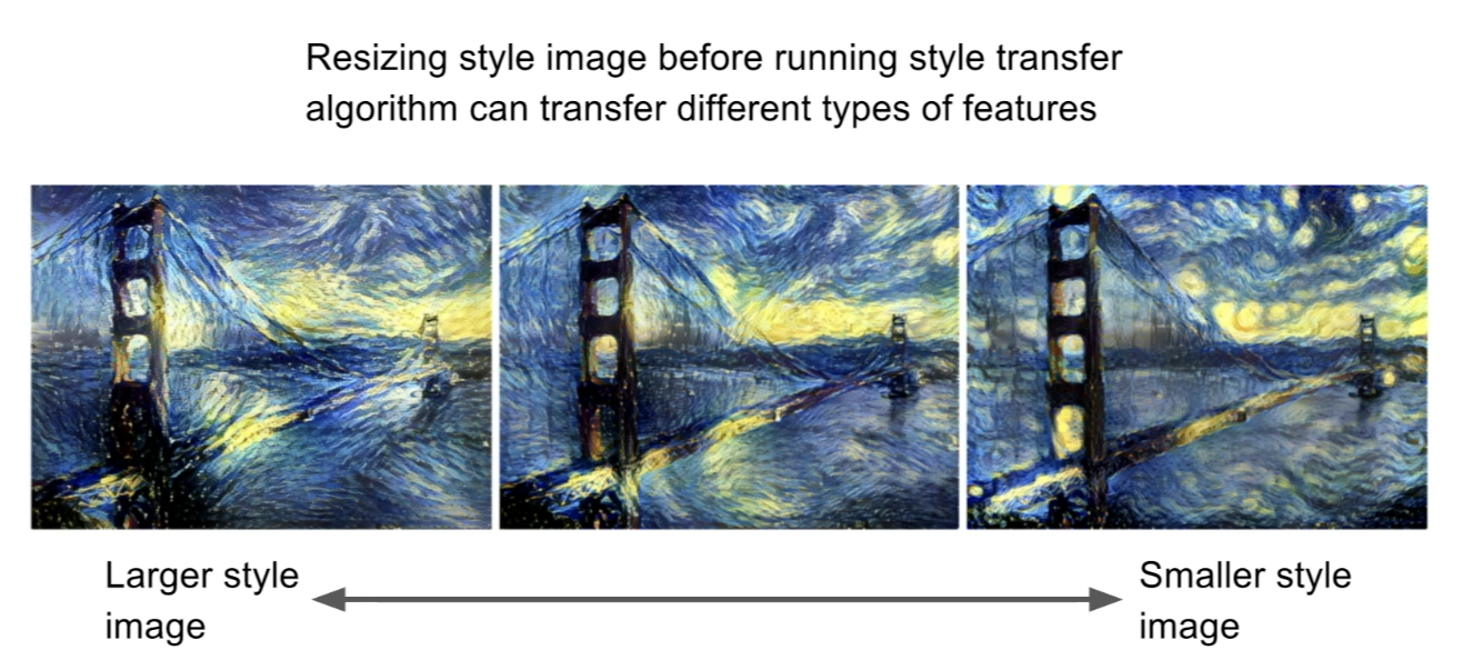
• resizing the style image before computing gram matrix
  - can get control over what the scale of features that you want to reconstruct from the style image is
  

Multiple Style Images

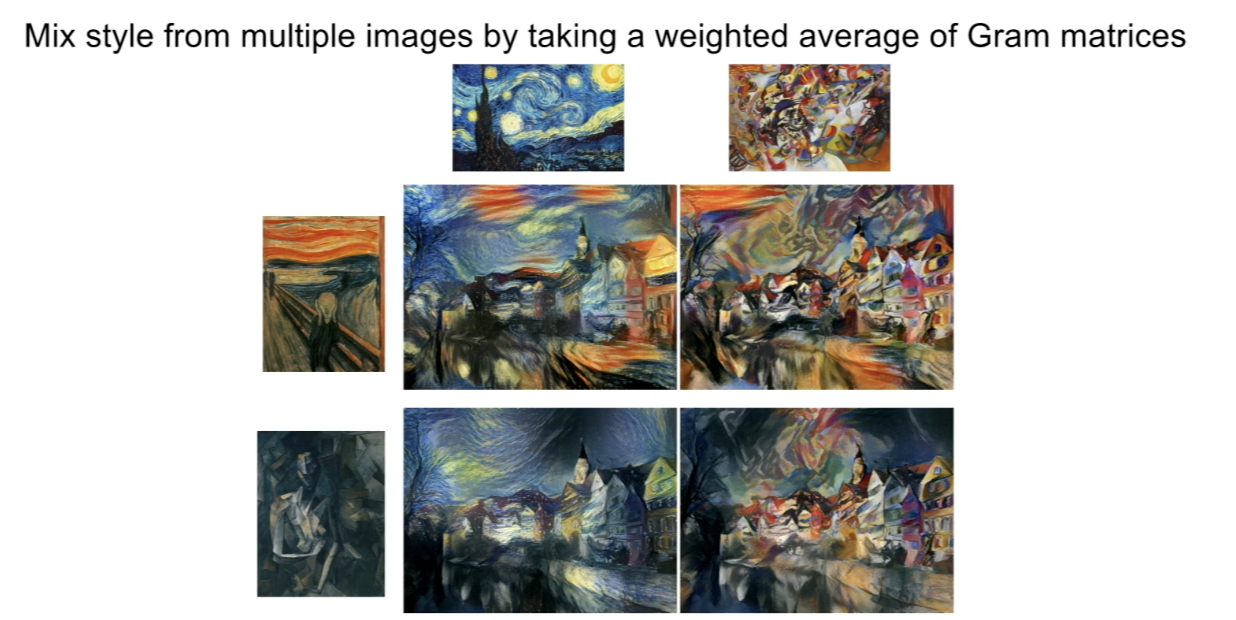
• match multiple gram matrices at the same time

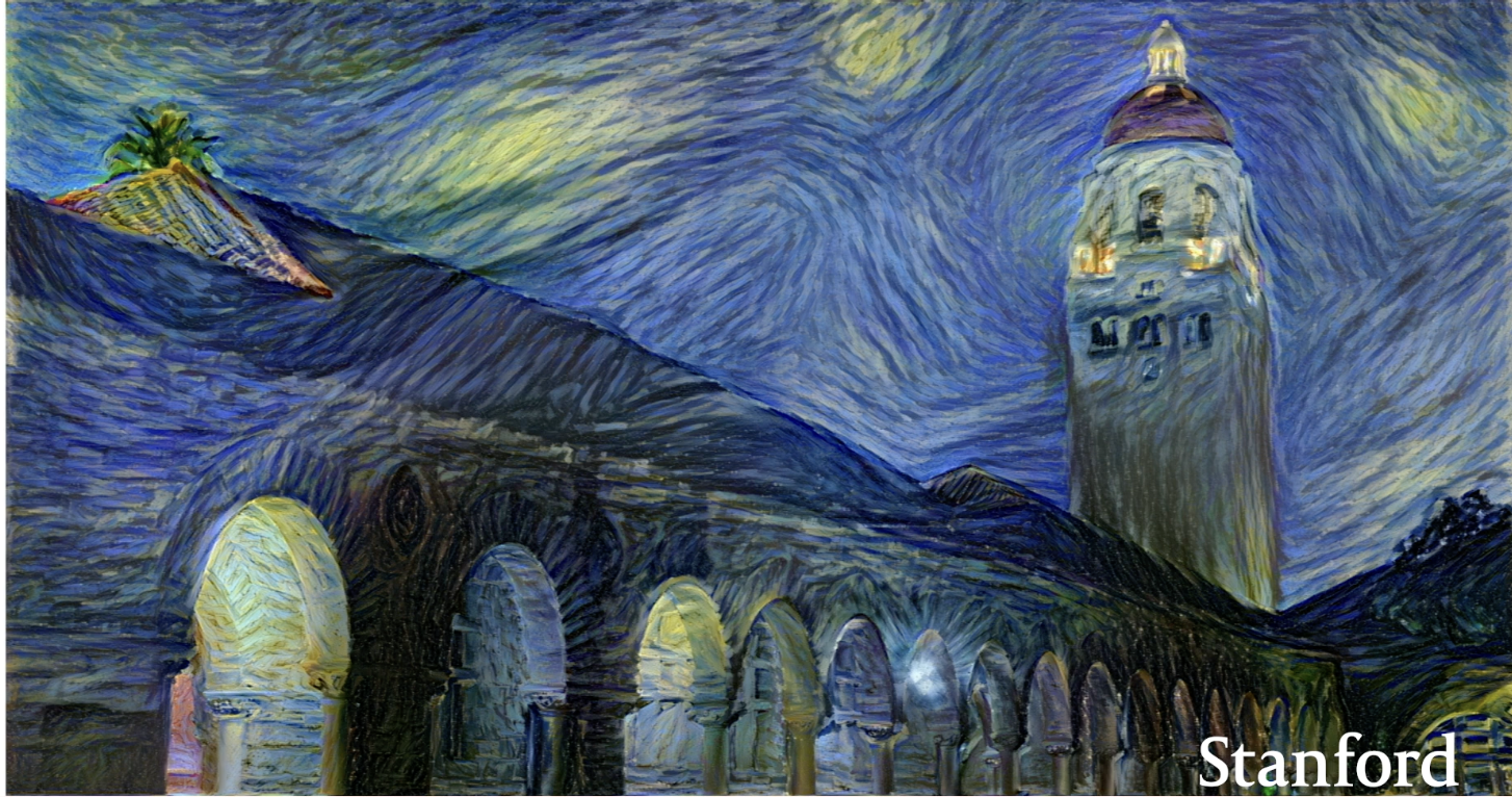
• if you do a multi-scale processing in style transfer
  - you can compute a very high resolution image
  • but very expensive to compute (took 4 GPUs)

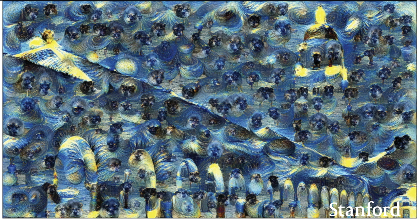
• you can joint style transfer and DeepDream at the same time
  - now we have 3 losses; content loss, style loss, and DeepDream loss(that tries to maximize the norm)

---

• problem: Style Transfer is pretty slow
  - you need to compute a lot of forward and backward passes through your pretrained network in order to compute images
• solution: train another neural network to perform style transfer
  - Fast Style Transfer

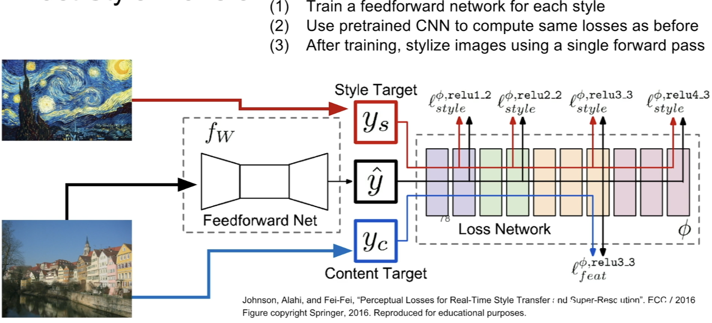
• fix some style that we care about at the beginning
• rather than running a separate optimization procedure for each image that we want to synthesize,
  - train a single feedforward network that can input the content image, and directly output the stylized result

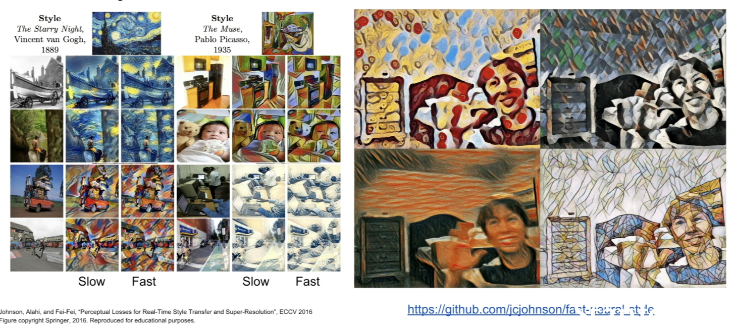
• train: compute the same content and style losses during training of feed forward network, and use that same gradient to update the weights of the feed forward network
• once it's trained, to produce stylized images, you just need to do a single forward pass through the trained network

Summary

• Many methods for understanding CNN representations
• Activations: Nearest Neighbors, Dimensionality reduction, maximal patches, occlusion
• Gradients: Saliency maps, class visualization, fooling images, feature invasion
• Fun: DeepDream, StyleTransfer