1. Introduction

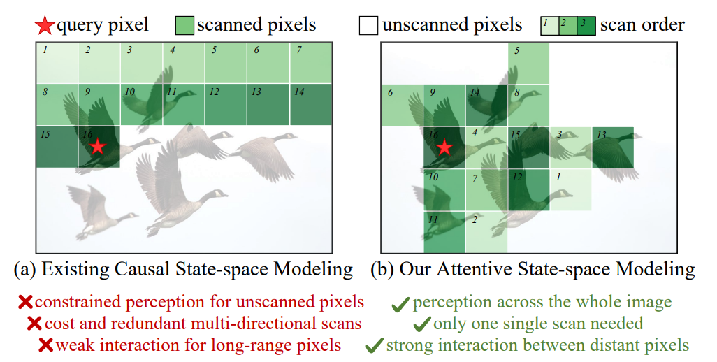
• Mamba-based methods의 “Causal State-Space Modelling”
  • 기존에는 정해진 scanning rule를 통해 2D 이미지를 1D token sequence로 unfold
  • Causal Property: 각 pixel은 scanned sequence 내 이전 pixel들에만 의존
  • Causal Property의 단점
    1. Undirectional Causality
    • Query pixel은 이전 pixel들로부터만 정보를 얻을 수 있고, 이후 pixel들은 인지할 수 없음
    • 이미지 전체에서 도움이 될 만한 픽셀을 충분히 활용하지 못함
    2. Necessity of Multi-Directional Scans
    • causal 특성으로 인해, multi-directional scan 필요
    • Multi-directional scan의 단점
      • 고해상도 입력에서 계산복잡도 크게 증가
      • 여러 방향 스캔으로 얻은 정보 사이에 중복이 꽤 있음
    3. Long-Range Decay
    • Mamba는 멀리 떨어진 토큰 간 상호작용이 약화됨
    • 중요하더라도 멀리 있다면, query pixel이 효과적으로 활용하지 못함

• 기존 Mamba의 단점: causal 특성 (이전 정보만 활용가능, 미래 토큰 활용 불가)
  • ViT의 non-causal 특성
    • query가 모든 key를 동시에 볼 수 있는 구조
    • 현재 토큰이 앞뒤 픽셀과 상호작용 가능
  • 제안: Mamba + ViT의 non-causal한 성질
    • Mamba의 문제는 causal 성질로 인해 뒤에 정보를 못 쓴다는 점
      ⇒ ViT의 non-causal 성질 사용하자!

• Attentive State-Space Restoration
  • ‘Attention의 Query’와 ‘State-Space Model의 Output Matrix(C)’는 구조적으로 유사하다는 점 활용
  • C를 Query처럼 사용하자!
    - 아직 스캔하지 않은 sequence의 “뒤쪽 토큰”까지 활용 → multi-directional scan의 필요성↓
    - 멀리 있지만 관련도가 높은 토큰을 1D 시퀀스에서 가깝게 재배치 → “의미적 유사도 기준으로 재정렬”
    
    

3 Key Contributions

1. Attentive State-space Equation (ASE)

• 방법
  • prompt가 의미적으로 비슷한 픽셀 집합을 대표하도록 설계
  • prompt를 state-space의 output matrix C에 residual addition 형태로 추가
• 효과
  • Mamba의 causal 성질로 인한 한계 완화
  • Single-pass scan만으로도 효율성을 높일 수 있음

2. Semantic Guided Neighboring (SGN)

• 방법
  • 각 픽셀에 semantic label 부여
  • label에 기반하여 semantic-neighboring 1D sequence 생성
  • 멀리 떨어져 있지만 의미적으로 비슷한 픽셀끼리의 상호작용 강화
• 효과
  • Mamba의 한계였던 long-range decay 문제 완화
  • 멀리 있는 픽셀들 간에도 효과적으로 상호작용할 수 있도록 만듦

3. MambaIRv2

• ASE + SGN + 기타 모듈
• Mamba의 state-space modeling + ViT의 non-causal capability
  
  
  
  

2. Related Work

• CNN의 한계
  • Convolution의 local kernel로 receptive field가 제한적
  • 멀리 떨어진 pixel 간 상호작용 ↓
• Transformer의 한계
  • 고해상도 이미지에서 비효율적
  • Input의 크기에 따라 계산복잡도가 2차로 증가
  • costly & impractical
    
    
• 효율적인 연산과 Global Receptive Field 간 균형 → “Mamba”를 IR 작업에 활용
• MambaIR의 한계
  • Local Pixel Forgetting : local 정보가 쉽게 사라지는 문제
  • Channel Redundancy : 채널 표현이 중복되는 문제
• FreqMamba
  • Fourier domain에서 SSM 적용
  • global degradation 인식 → image deraining 작업에 활용
• MambaLLIE
  • state space 방정식을 개선시켜, local 정보 강화
  • 저조도 영상 복원에 특화
    
    
• 여전히 Mamba의 Causality 문제 존재
  • Mamba의 causal modeling 특성으로 인해 한계 존재
  • 하지만 IR task는 non-causal task..
    
    
    
    

3. Motivation

Mamba-based Image Restoration

• Mamba는 토큰 간 상호작용을 ‘이산’ 상태공간 방정식으로 모델링

  State Space Equation adopted by Mamba

  

  $h_i = \bar{A} h_{i-1} + \bar{B} x_i$

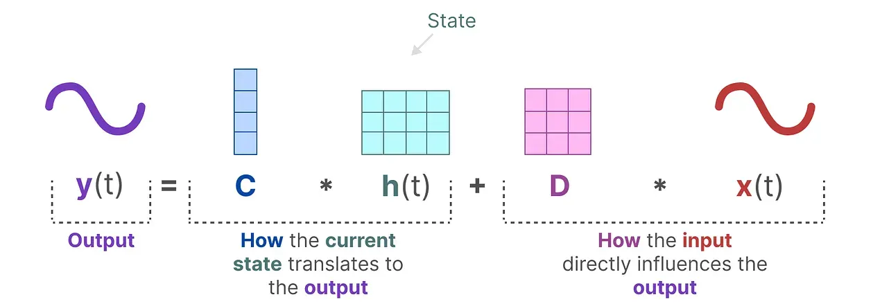
  • $\bar{A}$ : control matrix, $\exp(\Delta A)$
  • $\bar{B}$ : input matrix, $(\Delta A)^{-1}\left(\exp(\Delta A)-I\right)\Delta B \approx \Delta B$

  $y_i = \bar{C} h_i + D x_i$

  • $\bar{C}$ : output matrix

• $h_i$는 반드시 직전 상태인 $h_{i-1}$에 의존 → Causal(순차적) 구조
• i번째 토큰은 1,2,…,i−1 번째 입력에만 영향을 받음 = 과거 정보에만 영향을 받음
• Causal 특징의 장점
  • 시간/순서가 중요한 autoregressive task에는 유리함
• Causal 특징의 단점
  • non-causal task인 IR에서는 성능이 제한됨

Challenges from Causal Modeling

• 문제1 ) 2D → 1D scan

  
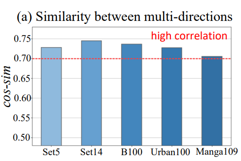
  • High Correlation with large rebundancy
  • 1D 시퀀스로 펴서 스캔을 하면, i번째 픽셀은 이전의 i-1개의 픽셀만 볼 수 있음
  • global context 활용 x
  • 해결 시도: Multi-directional scan
    • Multi-directional scan의 문제점
      • 여러 방향으로 스캔 → receptive field의 크기가 커짐 → 계산복잡도↑
      • 서로 다른 스캔 간 중복성이 큼

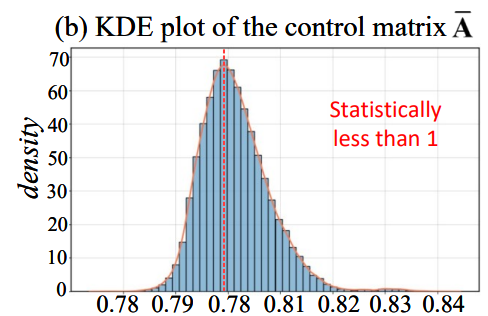
• 문제2) Long-range Decay

  

  • 멀리 떨어진 픽셀 간 정보 상호작용↓

  • $\bar{A}^k$ = interaction between pixels

  • Proof
    $h_0=\bar{B}x_0\\y_0=Ch_0+Dx_0$

    $h_1=\bar{A}h+\bar{B}x_1=\bar{A}\bar{B}x_0+\bar{B}x_1\\y_0=Ch_1+Dx_1=C(\bar{A}\bar{B}x_0+\bar{B}x_1)+Dx_1=C\bar{A}\bar{B}x_0+C\bar{B}x_1+Dx_1$

    [General Form]
    $y_k=C\bar{A^k}\bar{B}x_0 + C\bar{A^{k-1}}\bar{B}x_1 + ... + C\bar{B}x_k + Dx_k$

    

  • $C\bar{A^k}\bar{B}$ = contribution of $x_0$ to the generation of $y_k$

  • 입력 간 거리가 멀어질수록 (k가 커질수록), 영향력 감소 = long-range decay
    

4. Attentive State Space Restoration

4.1 Bridging Attention and State-Space

• 기존 Attetnion
  $\text{Attention}(Q, K, V) = \text{softmax}\left(\frac{QK^T}{\sqrt{d_k}}\right) V$
  • Query와 Key의 유사도 측정 → 유사도에 따라 가중치 부여 → 가중치로 Value 조합
  • Query-Key로 각 Value의 비율을 정함
• 기존 Attention의 문제: Softmax가 모든 j에 대해 한번에 계산해야함 → 비효율적
  
  
• Attention과 State Space 간의 강한 관계성이 있다고 판단해, Attention 과 State Space equation을 합치려는 시도
  • state = key-value의 누적합
  • query = state를 어떤 방식으로, selective 하게 읽을지 정함
    • output matrix C의 역할과 유사함
    • state의 projection

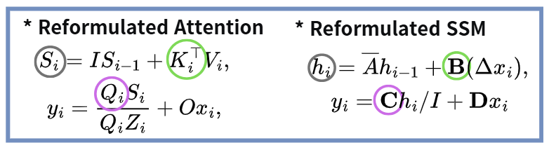
Reformulation of Attention

• Mamba가 linear complexity를 가진 causal model이기 때문에, “causal linear attention” 사용
• 기존 Causal Linear Attention
  • Formula: $y_i = \sum_{j=1}^i \frac{Q_i K_j^\top}{\sum_{t=1}^i Q_i K_t^\top} V_j= \frac{Q_i \left( \sum_{j=1}^i K_j^\top V_j \right)}{Q_i \left( \sum_{t=1}^i K_t^\top \right)}$
  • Denote : $S_i = \sum_{j=1}^i K_j^\top V_j, Z_i = \sum_{t=1}^i K_t^\top$
    • $S_i$ (state) = Key-Value의 누적합
    • $Z_i$ = 정규화 역할 , Key의 누적합
  • 재정의된 Causal Linear Attention 식: $y_i=Q_iS_i/Q_iZ_i$
  • 누적식 표현: $S_i = S_{i-1} + K_i^\top V_i, Z_i = Z_{i-1} + K_i^\top$
• Reformulated Form
  $S_i = I S_{i-1} + K_i^\top V_i, \\y_i = \frac{Q_i S_i}{Q_i Z_i} + O x_i ,$
  • $I$ : Identity Matrix
  • $O$ : Zero Matrix
  • $x_i$ : i번째 단계에서의 input token
  • Similar to SSM form
    $h_i=\bar{A}h_{i-1}+\bar{B}x_i \\ y_i=\bar{C}h_i+Dx_i$

Reformulation of State Space

• 기존 SSM 식
  $h_i = Ah_{i-1}+Bx_i \\ y_i=Ch_i+Dx_i$
  
• Reformulated Form
  $h_i = \overline{A} h_{i-1} + \mathbf{B}(\Delta x_i), \\ y_i = \mathbf{C} h_i / I + \mathbf{D} x_i .$
  • 연속 시간에서 정의된 SSM을 시간간격 Δ로 이산화
  • /I 는 attention 식과 형식을 맞추기 위해 표기

Connection Analysis

• SSM ↔ Attention 대응관계

  
  • 상태변수: $h_i​∼S_i​$
    • SSM의 hidden state ↔ Attention의 누적 상태
  • 입력: $B∼K^⊤$
    • SSM에서 입력 변환 행렬 B ↔ Attention의 key 역할
  • 출력: $C∼Q$
    • SSM의 출력 행렬 C ↔ Attention의 query 역할
  • CORE IDEA : C 행렬에 unscanned sequence의 정보를 넣어주는 것! ⇒ ASE 내 prompt
    - C를 Query처럼 사용
    - state 안에 encode된 unscanned/unseen 부분까지 끌어와
    - 현재 픽셀 복원 과정에 도움
    

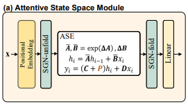
4.2. Attentive State Space Module

Attentive State Space Module

• MambaIRv2의 core block ← non-causal modeling with Mamba
• Modify output matrix $C\in\mathbb{R}^{L\times d }$ to globally query “related pixels across the image”
• Aim: original state-space equation of Mamba + non-causal nature
• What ASE do?
  • Incorporate prompts into C to supplement the missing information of the unseen pixels
  • Prompt = Set of pixels with similar semantics
    
    

PROMPT를 만드는 과정

1. Input Feature: $\mathbf{x} \in \mathbb{R}^{H \times W \times C}$
2. Positional Encoding : 기존 구조적 정보 보존하도록
3. SGN-unfold : 2D→1D
4. ASE(Attentive State-space Equation) modelling
   • 수정하고자 하는 부분: C
   • ‘Unseen pixel의 정보 보충 문제” ⇒ PROMPT를 C에 넣어줌
     • Prompt=비슷한 의미를 가진 pixel들의 set
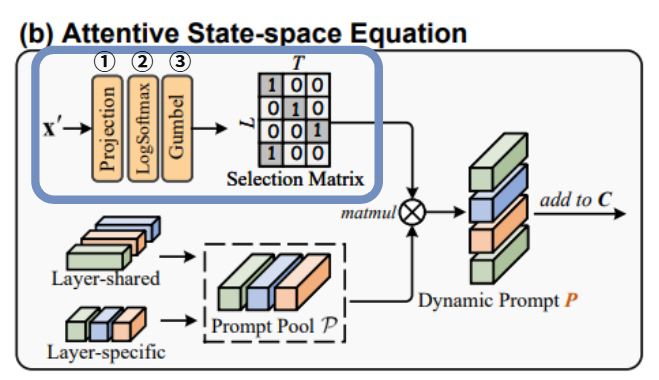
   • Prompt를 만드는 과정
     1) Prompt Pool 생성: $\mathcal{P}\in\mathbb{R}^{T\times d}$ (T=prompt의 개수)
     
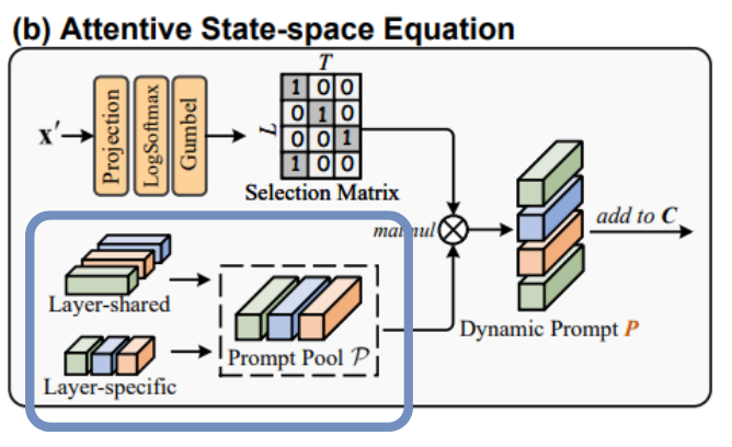
     2) $\mathcal{P}$의 Parameterization by ‘Semantic Decoupling’
     • Semantic Decoupling
       • 의미적으로 분리된 프롬프트 집합으로 설계
         $\mathcal{P}=MN , M \in \mathbb{R}^{T \times r},N \in \mathbb{R}^{r \times d}$
         • N = shared feature space
         • M = block-specific. combination coefficients
         • r = inner rank
       • 저차원 구조 공유(N) & block마다 다른 조합(M)
       • inner rank를 사용하는 이유
         • $\mathcal{P}$를 직접 학습하면 $T \times d$ 파라미터가 필요 → 너무 큼
         • $T⋅r+r⋅d≪T⋅d$ → M,N으로 분해하면 필요한 파라미터 수가 줄어듦
         • inner rank r: $\mathcal{P}$를 효율적이고 해석 가능하게 학습하기 위해 도입된 내부 잠재 차원
         • $\mathcal{P}$를 직접 크게 두는 대신 작은 r-차원 공간에서 factorization해,
           표현력을 유지하면서 파라미터 수를 줄이고, 공유 표현을 가능하게 함
     • 코드 확인

       self.embeddingB = nn.Embedding(num_tokens, inner_rank)   # [T, r]
       self.embeddingA = nn.Embedding(inner_rank, d_state)      # [r, d]
       full_embedding = self.embeddingB.weight @ token.weight   # [T, r] @ [r, d] = [T, d]

       • Prompt Pool : [T, d] = [num_tokens, d_state]
         • 저랭크 분해: P=B×A
           • $B \in \mathbb{R}^{T \times r}$ = embeddingB.weight
           • $A \in \mathbb{R}^{r \times d}$ = embeddingA.weight
     3) Routing Strategy
     

     • 프롬프트의 목적

       • degradation 관련 특징을 implicit하게 담음
       • degradation 유형의 클래스로 쓰이기보다는, 복원 prior/pattern의 학습된 basis

     • L=토큰 수=픽셀 수

       • L instance-specific prompts = 각 픽셀(토큰)마다 독립적인 프롬프트를 가짐

     • Routing Strategy

       • $\mathcal{P}$ 내에서 어떻게 선택할지 결정
       • Output: L개의 instance-specific prompts, $P \in \mathbb{R}^{L \times d}$
         • d=prompt vector 차원
       • 목적: C에 unscanned pixel의 정보 추가

     • 과정
       1) Flattened Input Feature: $\mathbf{x}' \in \mathbb{R}^{L\times C}$

       • L(픽셀 개수) * C(하나의 픽셀 내 feature channel)
       • Projection: C→T. prompt 개수로 project

       2) Linear Layer +LogSoftmax: $\mathbf{R} \in \mathbb{R}^{L\times T}$

       • Linear Layer
         • C → T(prompt의 개수)로 projection
       • LogSoftmax
         • 각 prompt별 log probability

       ①~②까지의 코드 확인

       self.route = nn.Sequential(
           nn.Linear(self.dim, self.dim // 3),  # 축소 + feature embedding
           nn.GELU(),                           # 비선형 활성화
           nn.Linear(self.dim // 3, self.num_tokens),  # ③ 최종 projection
           nn.LogSoftmax(dim=-1)                # log-prob 변환
       )
       
       pred_route = self.route(x)  # [B, L, T]

       • 첫번째 Linear(고차원 표현→compact embedding) → GELU(비선형 변환) → 두번째 Linear(압축된 표현→T개의 프롬프트 로짓) → LogSoftmax

       3) Gumbel-Softmax: $\mathbf{R} \in \mathbb{R}^{L\times T}$

       • 로그확률에 Gumbl noise를 더해 미분가능한 샘플링 진행
       • one-hot 선택에 가까운 Routing Matrix $R$

       ③ 코드 확인

       cls_policy = F.gumbel_softmax(pred_route, hard=True, dim=-1)  # [B, L, T]

       4) Instance-Specific Prompt: $\mathbf{P} \in \mathbb{R}^{L\times d}$

       • by matrix multiplication as $P=R\mathcal{P}$

       ④ 코드 확인

       prompt = torch.matmul(cls_policy, full_embedding)  # [B, L, d]
       # 토큰마다 선택된 프롬프트의 임베딩
       # cls_policy: [B, L, T] × full_embedding(=P): [T, d] -> [B,L,d] 

   • Prompt = Set of similar pixels
   • ASE의 장점
     • Attention-like Capability: query pixels across the whole image
     • unscanned pixel의 constrained perception 완화
     • 단방향 스캔으로 인한 높은 비용 / 여러방향 스캔으로 인한 중복 문제 X
5. SGN-fold: 1D→2D
6. Linear Projection
7. Output: Block Output
   
   

Semantic Guided Neighboring

• Problem

  • Causal modeling property of Mamba → Long-range decay
  • Existing Mamba-based Image SR의 여전한 문제점
    - weak utilization of the query pixel for scanned pixels which are spatially distant but similar
    - pixels that are distant in the original image are still far apart in the unfolded sequence
    
    

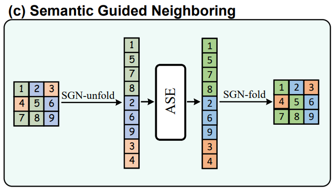
• Proposal : SGN(Semantic Guided Neighboring)

  • Image restoration = non-causal task & all pixels are observable at once
  • Re-define the token neighborhood to enable semantically similar tokens to be spatially closer in the unfolded sequence
  • Process
    1. 각 pixel 에 semantic label 부여 (semantic label = prompt category)
    2. SGN-unfold → 같은 semantic label을 가진 pixel들끼리 grouping으로 “Semantic-Neighbored Sequence” 생성
       • i-th prompt category → i-th semantic group
    3. SGN-fold (inverse transformation of SGN-unfold), to reshape back to spatial-space feature map, to obtain the output

4.3. Overall Network Architecture

• Mamba model은 global dependency를 잘 다루므로, “Local Interaction Modeling” 중요!
• Window MHSA(Multi-Head Self-Attention)를 활용해 위 문제 보완
  • 역할
    • window 내 local interactions
    • local patch 내에서만 self-attention 수행
  • MHSA의 문제는 높은 cost
    • ASSM의 단방향 scan으로 남는 parameter budget으로 Local MHSA를 넣겠다는 아이디어
    • MHSA는 cost가 높지만, window attention은 크기가 제한돼, 효율적으로 사용 가능

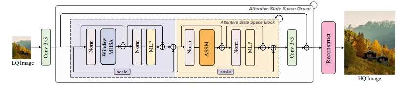
1. 3×3 Convolution Layer → Shallow Feature
2. Shallow Feature는 ASSG에 들어감
   2-1) ASSG = ASSB 여러개를 모아둔 단위
   2-2) ASSB
   • Local-to-Global Modeling to form the image hierarch
   • Transformer 구조 베이스 + token mixer 자리에 Window MHSA(local)/ASSM(global)
3. Task-specific Reconstruction Modules
   • e.g., pixelshuffle for SR, convolution for DN

5. Experiments

• Tasks

  1. Super-Resolution (SR)
     • classic SR
     • lightweight SR
  2. JPEG Compression Artifact Reduction (JPEG CAR)
  3. Gaussian Color Image Denoising

• Experimental Settings

  • Data Augmentation : Horizontal Flip, Random Rotation of 90°, 180°, 270°
  • Crop: 64×64(SR) , 128×128(DN)
    
    
  • Optimizer: Adam (β₁=0.9, β₂=0.999)
  • Loss
    • L1 Loss → SR
    • Charbonnier Loss → Denoising / JPEG CAR
  • Learning Rate
    • 초기값: 2 × 10⁻⁴
    • 특정 iteration에서 half decay

5.2 Ablation Study

Ablations with MambaIRv2-light 2× SR model trained for 250K iterations on the DIV2K dataset

Effectiveness of Different Components

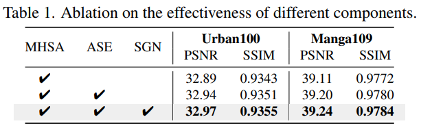
1. ASSM- (= pure Attention variant)
   • only use window attention → limit receptive field to the local window → limit performance
2. ASSM+ SGN- (= Only ASE)
   • query of similar pixels across images → improve performance by 0.05 dB/0.09 dB in Urban100/Manga109
3. Proposed Method
   • effectively overcome the long-range decay of Mamba
   • best performance of 32.97/39.24 dB PSNR on Urban100/Manga109

Abalation on Attentive State-space Equation

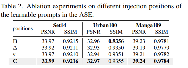
• Inserting Positions of the Prompts in ASE
  • B → decent results, but slightly inferior to adding to C ⇒ “C is closer to the output end in the state-space equation”
  • time-step ∆, output y → fail to give satisfactory performance

5.3. Comparison on Image Super-Resolution

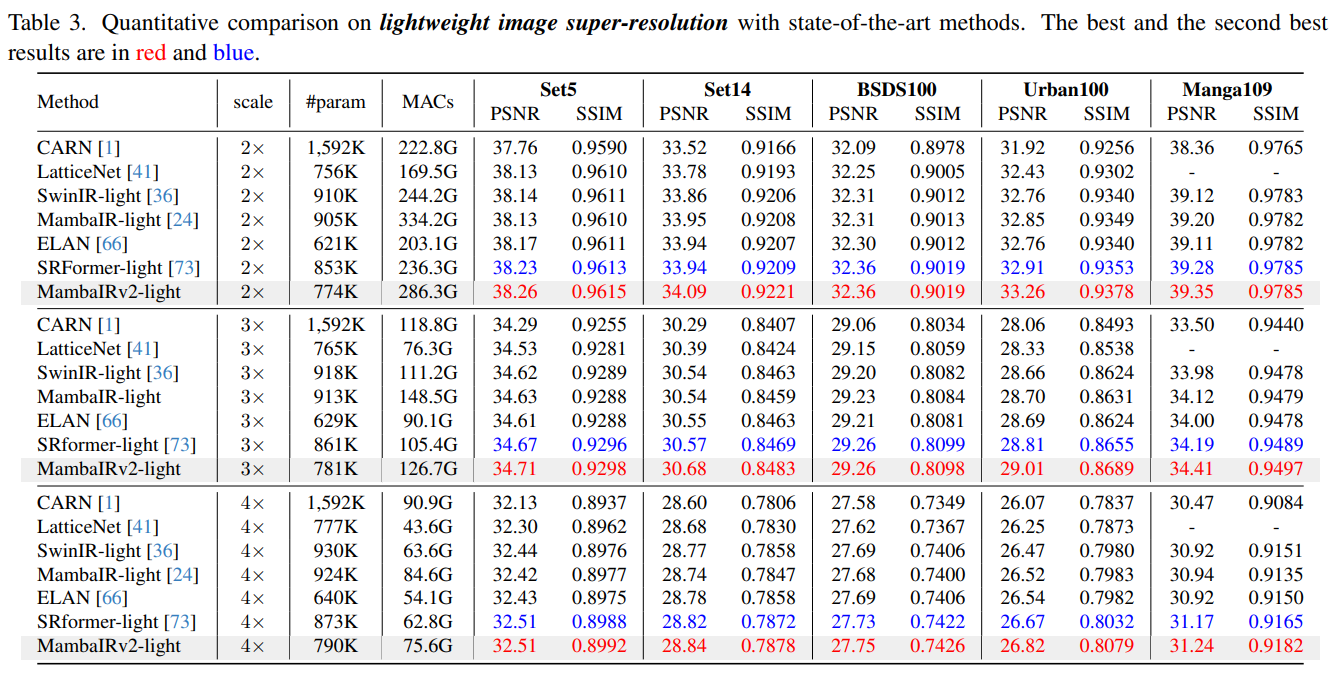
Lightweight Image Super-Resolution

Classic Image Super-Resolution

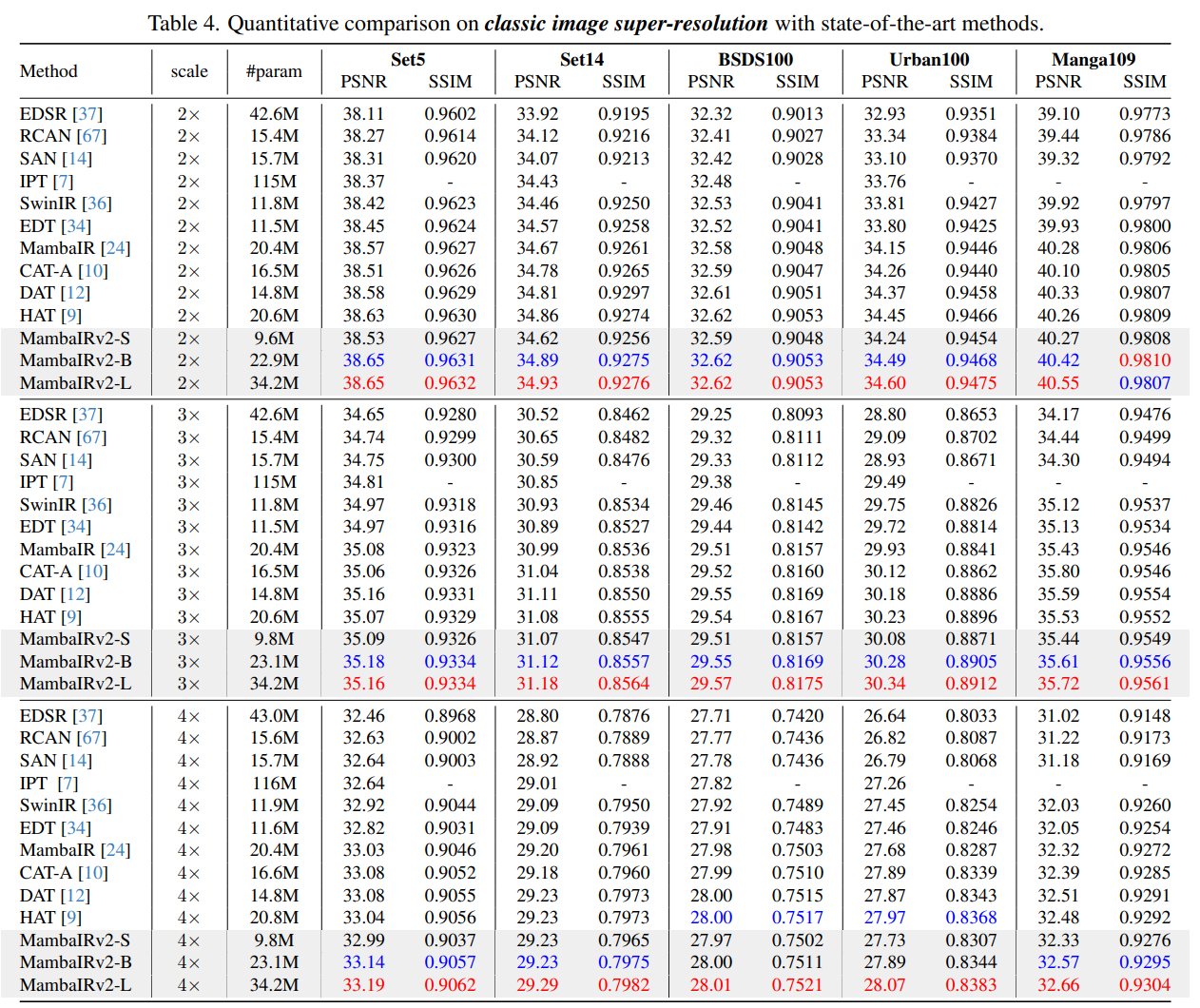
• Results of Comparison of MambaIRv2 with different model sizes
• Thanks to ASSM, MambaIRv2 achieved best performance across most 5 benchmark dataset and up-sample scales
• Balance of performance and efficiency
  • Higher Performance & Fewer Parameter

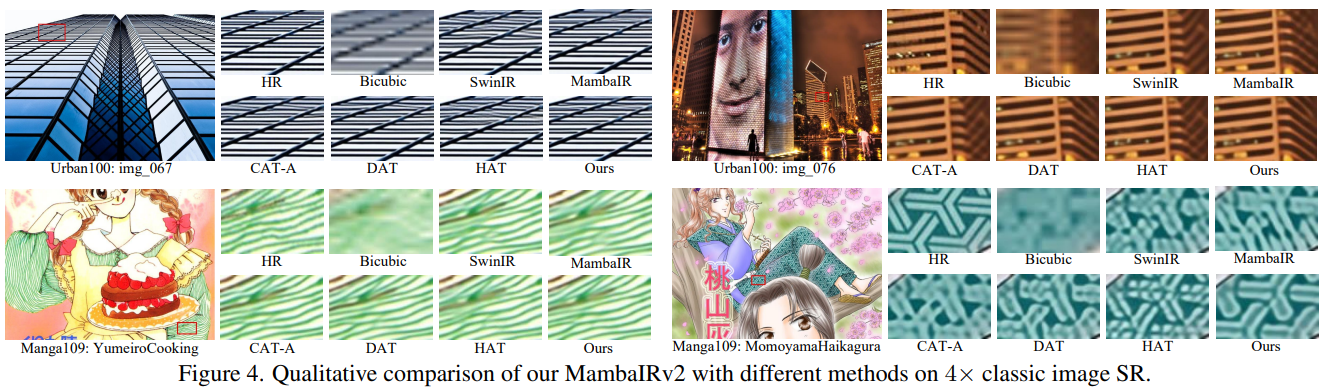
Model Complexity Comparison

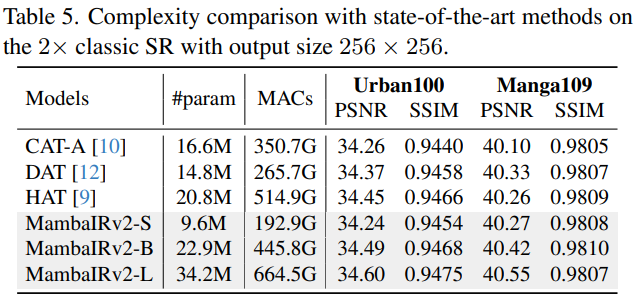
• MambaIRv2-S model vs CAT-A
  • use 55.0% of the MACs & outperform by 0.17dB PSNR on Manga109
• MambaIRv2-B model vs HAT
  • roughly matches the #param & 13.4% reduction in MACs
  • 0.04/0.16dB PSNR improvements on Urban100/Manga109
• MambaIRv2 strikes a sweet spot between performance and efficiency

5.4. Comparison on JPEG CAR

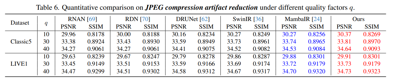
• MambaIRv2 achieves the best performance on all testing datasets across all quality factors
• (ex) MambaIRv2 suppresses MambaIR by 0.11dB PSNR with q = 40 on the Classic5 datasets

5.5. Comparison on Image Denoising

• 서로 다른 restoration task 간의 일관성을 유지하기 위해, straight-through structure 활용. UNet구조 사용 X
  • UNet 구조는 DN task에 매우 유리한 구조

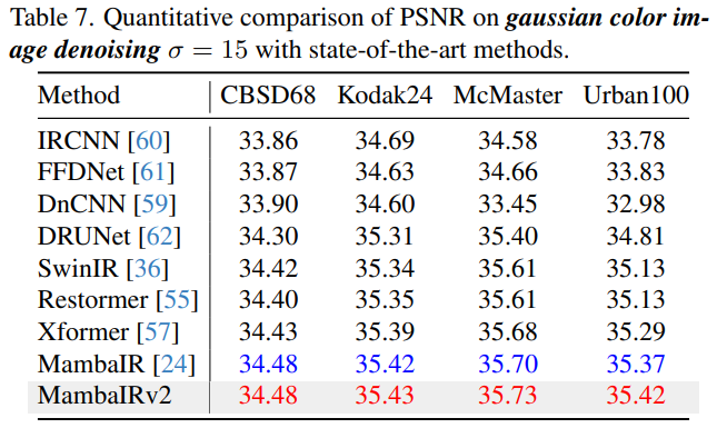
• MambaIRv2 outperforms all other models across the datasets
• In particular, it surpasses U-shaped Restormer by even 0.29dB PSNR on the Urban100 dataset
• This experiment validates our MambaIRv2 serves as a generalized image restoration backbone

5.6. Discussion

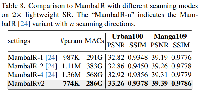
Benefits from Reduced Scan Directions

• Compared to MambaIR, which performs 4 scans in pixel space,
  • significant advantage of our MambaIRv2 is that it requires only a single scan in the semantic space
• MambaIRv2 : efficient + higher performance
  • reduces 43% of #param, 50% computational burden
  • while still suppresses by 0.34dB PSNR on 2× Urban100

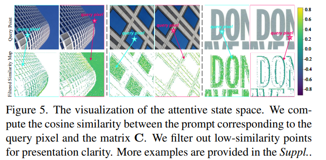
Visualization of Attentive State Space

• Prompts in ASSE : similar pixels across the whole image to facilitate the query pixel seeing out of the scanned sequence
• Query pixel is empowered to attend to its corresponding semantic part in the image through the prompt → enable global information aggregation

6. Conclusion

• Problem: Causal modeling nature of Mamba
• Proposal
  • Attentive State-Space Equation → incorporates prompt learning for enlarged token perception as well as scanning only once
  • Semantic Guided Neighboring → positions similar pixels closer to handle the long-range decay
• MambaIRv2
  • ViT-like non-causal abilities ⊕ Mamba-based models → implement the attentive state space restoration
  • Extensive experiments confirm our MambaIRv2 as an efficient, highperforming backbone for image restoration