멀티캠퍼스 데이터분석 5월 22일 수업 내용 — RNN 이론, DataLoader, ANN 회귀 vs XGBoost 비교 실습, RNN sin 곡선 예측 실습

---

📌 목차

이론
1. 시계열 데이터와 RNN
2. RNN 핵심 구조 & 수학적 원리
3. RNN 매개변수 정리
4. DataLoader — 배치 단위 데이터 공급

실습

5. 연습문제 — ANN 회귀 vs XGBoost (insurance 데이터)
6. RNN 실습 — sin 곡선 시계열 예측

---

이론

1. 시계열 데이터와 RNN

시계열 데이터 (Time-Series Data)

주식 가격, 날씨, 센서값처럼 시간의 흐름에 따라 순서대로 기록된 데이터를 의미합니다.

💡 주식 차트 비유
오늘 하루의 가격표만 보고 내일의 주가를 맞출 수 없습니다.
한 달 전부터 어제까지 이어져 온 상승/하락 추세를 기억해야 흐름을 이해할 수 있습니다.

RNN의 역할

과거의 패턴 정보를 내부에 기억하고, 이를 다음 시점의 분석으로 계속 전달해 주는 시계열 특화 딥러닝 모델입니다.

RNN 산업별 시계열 활용 사례

---

2. RNN 핵심 구조 & 수학적 원리

핵심 구조 — 시간의 흐름을 잇는 은닉 상태

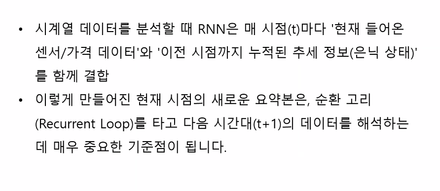
• 첫 번째 입력 → 초기 상태 h_0 = 0 과 입력으로 h_1 계산
• 두 번째 입력 → 이전 상태 h_1 과 결합하여 h_2 계산
• 세 번째 입력 → 이전 상태 h_2 와 결합하여 h_3 계산
• 반복 완료 → 마지막 상태 h_t 생성 (모든 과거 정보를 결합한 상태)

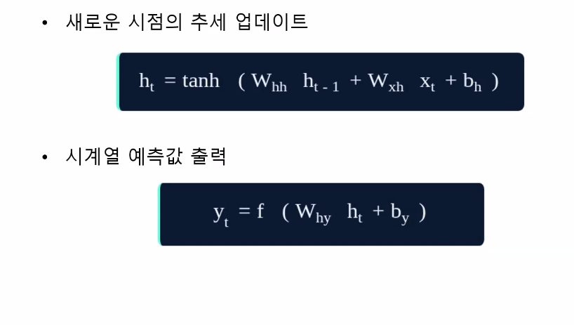
RNN 수학적 작동 원리

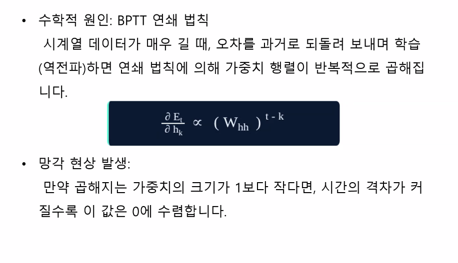
RNN의 한계 — 기울기 소실과 망각

---

3. RNN 매개변수 정리

주요 매개변수

매개변수	기본값	설명
input_size	-	각 시점에서 입력 피처의 수
hidden_size	-	은닉층(출력)의 크기
num_layers	1	RNN 층의 개수 (깊어질수록 복잡한 패턴, 과적합 위험)
nonlinearity	'tanh'	비선형 활성화 함수
batch_first	False	True 시 입력 형태 → (배치, 구간, 피처)
bias	True	각 가중치에 편향 항 추가 여부
dropout	0.0	층 사이 Dropout 비율 (층이 2개 이상인 경우에만 사용)
bidirectional	False	양방향 RNN 사용 여부

매개변수 설정 가이드

매개변수	권장 범위	주의사항
hidden_size	32, 64, 128	너무 작으면 정보 부족, 너무 크면 과적합
num_layers	1 ~ 3	1부터 테스트하여 교차 검증
nonlinearity	'tanh' 권장	'relu' 사용 시 속도 빠르나 발산 위험
dropout	0.2 ~ 0.5	층이 2개 이상인 경우에만 사용

---

4. DataLoader — 배치 단위 데이터 공급

PyTorch에서 Dataset을 효율적으로 배치 단위로 꺼내주는 반복자입니다.

from torch.utils.data import DataLoader

train_dl = DataLoader(
    train_ds,
    batch_size = 64,    # Dataset을 묶어서 텐서로 제공
    shuffle    = True,  # 에폭마다 데이터 순서를 랜덤하게 변경
    drop_last  = True,  # 마지막 배치가 batch_size보다 작으면 제거
    # pin_memory = True  # GPU 사용 시 CPU→GPU 전송 속도 향상
)

DataLoader 주요 매개변수

매개변수	설명
batch_size	한 번에 묶어서 처리할 샘플 수
shuffle	에폭마다 데이터 순서를 랜덤하게 변경
drop_last	마지막 배치 크기가 작으면 제거
pin_memory	GPU 사용 시 CPU→GPU 전송 속도 향상

---

실습

5. 연습문제 — ANN 회귀 vs XGBoost (insurance 데이터)

문제 정의

insurance.csv 데이터에서 charges(보험료)를 예측합니다.

• 딥러닝: PyTorch 다중 퍼셉트론 (Epoch 300)
• ML: XGBoost + GridSearchCV
• 비교 지표: R² Score

데이터 로드 & 컬럼 설명

import pandas as pd
from sklearn.model_selection import train_test_split, GridSearchCV, KFold
from sklearn.metrics import r2_score
from sklearn.preprocessing import StandardScaler
from sklearn.pipeline import Pipeline
from xgboost import XGBRegressor
import torch
import torch.nn as nn
import torch.optim as optim

df = pd.read_csv('../data/insurance.csv')

컬럼	설명
age	나이
sex	성별
bmi	체질량 지수
children	자녀 수
smoker	흡연 여부
region	거주 지역
charges	보험료 ← target

전처리

# 범주형 데이터 더미화
df = pd.get_dummies(df, columns=['sex', 'smoker', 'region'], drop_first=True)

x = df.drop('charges', axis=1)
y = df['charges']

X_train, X_test, y_train, y_test = train_test_split(
    x, y, test_size=0.2, random_state=42
)

ANN 회귀 모델 — PyTorch 다중 퍼셉트론

# 스케일링 & Tensor 변환
scaler      = StandardScaler()
X_train_sc  = scaler.fit_transform(X_train)
X_test_sc   = scaler.transform(X_test)

X_train_tensor = torch.tensor(X_train_sc, dtype=torch.float32)
X_test_tensor  = torch.tensor(X_test_sc,  dtype=torch.float32)

# 1차 행렬 → 2차 행렬 변환 (종속 변수)
# 방법 1 — reshape(-1, 1)
y_train_tensor = torch.tensor(y_train.values.reshape(-1, 1), dtype=torch.float32)
y_test_tensor  = torch.tensor(y_test.values.reshape(-1, 1),  dtype=torch.float32)

# 방법 2 — unsqueeze(-1)
y_train_tensor2 = torch.tensor(y_train.values, dtype=torch.float32).unsqueeze(-1)

# 방법 3 — view(-1, 1)  (numpy의 reshape과 유사)
y_train_tensor3 = torch.tensor(y_train.values, dtype=torch.float32).view(-1, 1)

💡 1차 → 2차 행렬 변환 방법 3가지 비교

방법	코드	특징
reshape(-1, 1)	numpy 단계에서 변환 후 tensor 생성	가장 일반적
.unsqueeze(-1)	tensor 생성 후 마지막 차원 추가	PyTorch 스타일
.view(-1, 1)	tensor 생성 후 형태 변경	numpy reshape과 유사

# 모델 정의 — Dropout 포함 다층 퍼셉트론
class Reg_Model(nn.Module):
    def __init__(self, _dim):
        super(Reg_Model, self).__init__()
        self.model = nn.Sequential(
            nn.Linear(_dim, 64),
            nn.ReLU(),
            nn.Dropout(0.2),   # 과적합 방지
            nn.Linear(64, 32),
            nn.ReLU(),
            nn.Dropout(0.2),
            nn.Linear(32, 1)
        )
    def forward(self, x):
        return self.model(x)

model     = Reg_Model(X_train_tensor.shape[1])
criterion = nn.MSELoss()
optimizer = optim.Adam(model.parameters(), lr=0.01)

# 학습
for epoch in range(300):
    pred = model(X_train_tensor)
    loss = criterion(pred, y_train_tensor)

    optimizer.zero_grad()
    loss.backward()
    optimizer.step()

    if (epoch + 1) % 30 == 0:
        print(f'Epoch {epoch+1}/300, Loss: {round(loss.item(), 6)}')

# 평가
model.eval()
with torch.no_grad():
    pred = model(X_test_tensor)
    r2   = r2_score(y_test_tensor, pred)
    print(f'R2 Score : {round(r2, 5)}')
    print(f'예측값: {pred[0]}, 실제값: {y_test_tensor[0]}')

💡 nn.Dropout(p)
학습 중 p 비율의 뉴런을 랜덤하게 비활성화하여 과적합을 방지합니다.
model.eval() 시에는 자동으로 비활성화됩니다.

XGBoost — Pipeline + GridSearchCV

pipe = Pipeline([
    ('std', StandardScaler()),
    ('xgb', XGBRegressor(random_state=42))
])

params = {
    'xgb__n_estimators'  : [100, 200, 300],
    'xgb__learning_rate' : [0.01, 0.05, 0.1],
    'xgb__max_depth'     : [3, 4, 5],
    'xgb__subsample'     : [0.8, 0.9, 1.0]
}

cv = KFold(n_splits=5, shuffle=True, random_state=42)

grid = GridSearchCV(
    pipe,
    param_grid = params,
    cv         = cv,
    n_jobs     = -1,
    scoring    = 'r2'
)

grid.fit(X_train, y_train)

print('Best Params :', grid.best_params_)

pred = grid.predict(X_test)
print(f'R2 Score : {round(r2_score(y_test, pred), 4)}')
print(f'예측값: {pred[0]}, 실제값: {y_test.values[0]}')

---

6. RNN 실습 — sin 곡선 시계열 예측

데이터 생성 — 노이즈 포함 sin 곡선

import math
import numpy as np
import torch
import torch.nn as nn
import torch.optim as optim
from torch.utils.data import DataLoader, Dataset
from sklearn.preprocessing import StandardScaler
import matplotlib.pyplot as plt

np.random.seed(42)
torch.manual_seed(42)

# 노이즈가 포함된 sin 곡선 생성
x = torch.arange(3000).float()
y = torch.sin(2 * math.pi * 0.02 * x) + 0.05 * torch.randn(3000)

plt.figure(figsize=(20, 13))
plt.plot(x, y)
plt.show()

데이터 분할 & 스케일링 & Tensor 변환

train_size = int(0.8 * len(x))   # 앞 80% → train

X_train = y[:train_size]
X_test  = y[train_size:]

scaler       = StandardScaler()
X_train_sc   = scaler.fit_transform(X_train.reshape(-1, 1))
X_test_sc    = scaler.transform(X_test.reshape(-1, 1))

X_train_tensor = torch.tensor(X_train_sc, dtype=torch.float32)
X_test_tensor  = torch.tensor(X_test_sc,  dtype=torch.float32)

# (N, 1) → (1, N, 1) : 배치 차원 추가
X_train_tensor = X_train_tensor.unsqueeze(0)
X_test_tensor  = X_test_tensor.unsqueeze(0)

print(X_train_tensor.shape)   # (1, 2400, 1)

💡 unsqueeze(0) — 0번 차원(배치 차원)을 추가합니다.
(2400, 1) → (1, 2400, 1) : (배치 크기, 시퀀스 길이, 피처 수)

RNN 모델 정의

class RNN_Model(nn.Module):
    def __init__(self):
        super(RNN_Model, self).__init__()
        self.rnn = nn.RNN(
            input_size    = 1,
            hidden_size   = 64,
            num_layers    = 1,
            batch_first   = True,
            dropout       = 0.0,
            nonlinearity  = 'tanh',
            bidirectional = False
        )
        self.linear = nn.Linear(64, 1)

    def forward(self, x):
        # out  : 모든 시점의 은닉층 값
        # h_n  : 마지막 시점의 은닉층 값
        out, h_n = self.rnn(x)
        result   = self.linear(h_n[-1])   # 마지막 층의 은닉 상태 사용
        return result

WindowDataset & DataLoader

class WindowDataset(Dataset):
    def __init__(self, _data, _window):
        self.data   = _data
        self.window = _window
        self.n      = len(self.data) - self.window

    def __len__(self):
        return self.n

    def __getitem__(self, idx):
        # 입력: idx 부터 window 크기만큼의 구간
        x = self.data[idx : idx + self.window]
        # 정답: window 이후 다음 시점
        y = self.data[idx + self.window]
        return x, y

window   = 10
train_ds = WindowDataset(X_train_tensor.squeeze(0), window)

train_dl = DataLoader(
    train_ds,
    batch_size = 64,
    drop_last  = True,
    shuffle    = True
)
test_dl = DataLoader(
    WindowDataset(X_test_tensor.squeeze(0), window),
    batch_size = 64,
    drop_last  = True,
    shuffle    = True
)

학습 루프

model     = RNN_Model()
criterion = nn.MSELoss()
optimizer = optim.Adam(model.parameters(), lr=0.01)

train_loss_list = []

for epoch in range(20):
    model.train()
    running, n_seen = 0.0, 0

    for x, y in train_dl:
        x, y = x.float(), y.float()

        yhat = model(x)
        loss = criterion(yhat, y)

        optimizer.zero_grad()
        loss.backward()
        torch.nn.utils.clip_grad_norm_(model.parameters(), 1.0)
        optimizer.step()

        running += loss.item() * x.size(0)
        n_seen  += x.size(0)

    train_loss = running / max(1, n_seen)
    train_loss_list.append(train_loss)
    print(f'Epoch {epoch+1}, Train Loss: {round(train_loss, 8)}')

# 학습 곡선 시각화
plt.plot(train_loss_list)
plt.grid()
plt.show()

예측값 vs 실제값 시각화

model.eval()
preds, trues = [], []

with torch.no_grad():
    for x, y in test_dl:
        x, y = x.float(), y.float()
        pred = model(x)
        preds.append(pred)
        trues.append(y)

preds = torch.cat(preds, 0).squeeze(-1).numpy()
trues = torch.cat(trues, 0).squeeze(-1).numpy()

plt.figure(figsize=(20, 13))
plt.plot(preds[:100], label='Predicted')
plt.plot(trues[:100], label='True')
plt.legend()
plt.grid()
plt.show()

---

📎 핵심 개념 요약

개념	설명
시계열 데이터	시간 순서대로 기록된 데이터
RNN	이전 시점의 은닉 상태를 다음 시점에 전달하는 순환 신경망
h_n	마지막 시점의 은닉 상태 — 모든 과거 정보 압축
batch_first=True	입력 형태를 (배치, 구간, 피처) 순서로 지정
bidirectional=True	순방향 + 역방향 양쪽으로 학습 (hidden_size 2배)
dropout	층이 2개 이상일 때만 사용, 과적합 방지
nn.Dropout(p)	학습 중 p 비율 뉴런 랜덤 비활성화
.unsqueeze(0)	0번 차원(배치)을 추가
.unsqueeze(-1)	마지막 차원을 추가
.view(-1, 1)	tensor 형태 변경 (numpy reshape과 유사)
reshape(-1, 1)	numpy 배열 형태 변경
torch.manual_seed(42)	PyTorch 랜덤 시드 고정
np.random.seed(42)	numpy 랜덤 시드 고정
WindowDataset	시계열을 window 구간(x)과 다음 시점(y)으로 분리
drop_last=True	마지막 배치가 batch_size보다 작으면 제거
pin_memory=True	GPU 사용 시 데이터 전송 속도 향상
Pipeline + GridSearchCV	스케일러 + 모델을 하나로 묶어 최적 파라미터 탐색
KFold	K겹 교차 검증 (시계열이 아닌 경우 shuffle=True)