DBSCAN & 금융 데이터 분석 & 주식 데이터 실습 정리

1. 핵심점 생성  → 각 점의 이웃 개수 계산 (반경 eps 내 min_samples 이상이면 핵심점)
2. 경계점 생성  → 핵심점 근처에 있지만 자신은 핵심점이 아닌 경우
3. 노이즈점 생성 → 어떠한 군집에도 속하지 않는 데이터
4. 군집 확장   → 핵심점에서 시작해 이웃을 계속 측정하며 확장

주요 매개변수

매개변수	기본값	설명
`eps`	`0.5`	같은 군집으로 간주할 최대 거리(반경)
`min_samples`	`5`	핵심점 판단을 위한 최소 샘플 수
`metric`	`'euclidean'`	거리 계산 방식
`algorithm`	`'auto'`	이웃 탐색 알고리즘
`leaf_size`	`30`	Tree 알고리즘 사용 시 리프 크기
`n_jobs`	`None`	병렬 CPU 수

algorithm 옵션

값	설명
`'auto'`	데이터 특성에 따라 자동 선택
`'brute'`	모든 점 간 거리 계산 (데이터가 적을 때)
`'kd_tree'`	20차원 이하 저차원 데이터에서 빠름
`'ball_tree'`	고차원 데이터에서 효율적

주요 속성

속성	설명
`labels_`	각 데이터의 군집 라벨 (노이즈는 -1)
`core_sample_indices_`	핵심점의 인덱스 목록
`components_`	핵심점 좌표 배열

파라미터 튜닝 팁

문제 상황	해결 방법
노이즈가 너무 많다	`eps` 증가 or `min_samples` 감소
군집이 너무 뭉친다	`eps` 감소
고차원 데이터	차원 축소 후 사용
속도가 느리다	`algorithm='kd_tree'` or `n_jobs=-1`

2. DBSCAN 실습 — bodyPerformance 데이터

데이터 로드 & 전처리

import numpy as np
import pandas as pd
import matplotlib.pyplot as plt
from sklearn.preprocessing import StandardScaler, LabelEncoder
from sklearn.cluster import DBSCAN
from sklearn.neighbors import NearestNeighbors
from sklearn.metrics import silhouette_score, adjusted_rand_score
from sklearn.decomposition import PCA

df = pd.read_csv('../data/bodyPerformance.csv')

# 범주형 컬럼 LabelEncoding
obj_cols = df.select_dtypes('object').columns
le = LabelEncoder()
for col in obj_cols:
    df[col] = le.fit_transform(df[col])

x  = df.drop(['class'], axis=1)
y1 = df['class']
y2 = df['gender']

x_std = StandardScaler().fit_transform(x)

NearestNeighbors로 최적 eps 탐색

# k번째 최근접 이웃의 거리 계산
nbrs = NearestNeighbors(n_neighbors=10).fit(x_std)
distances, idxs = nbrs.kneighbors(x_std)

# 10번째 이웃의 거리만 추출하여 정렬
kth_list = np.sort(distances[:, -1])

plt.figure(figsize=(10, 8))
plt.plot(kth_list)
plt.grid(True)
plt.show()

💡 eps 결정 방법 — 꺾이는 지점(Elbow Point)
그래프에서 기울기 변화가 가장 큰 지점이 최적 eps입니다.
np.diff() 로 변화량을 계산하고, 급변하는 인덱스를 찾으면 됩니다.

# 기울기 급변 지점 탐색
diffs = np.diff(kth_list)
eps_ = np.where(diffs > 0.05)[0]

print('급변하는 인덱스 :', eps_)
print('대략적인 최적 eps :', kth_list[eps_[0]])

DBSCAN 학습 & 검증

db = DBSCAN(eps=1.7, min_samples=10, n_jobs=-1)
labels = db.fit_predict(x_std)

# 군집 종류 확인
print(set(labels))

# 노이즈 개수 확인
print('노이즈 개수 :', np.sum(labels == -1))

# 검증 지표 (노이즈 제외)
flag = labels != -1
sil = silhouette_score(x_std[flag], labels[flag])
ari = adjusted_rand_score(y2, labels)

print('Silhouette :', sil)
print('ARI        :', ari)

PCA 2차원 축소 후 군집 시각화

pca = PCA(n_components=2, random_state=42)
x_pca = pca.fit_transform(x_std)

non_noise = labels != -1

# 비노이즈 데이터
plt.scatter(x_pca[non_noise, 0],  x_pca[non_noise, 1],
            c=labels[non_noise], cmap='tab10', label='Cluster', alpha=0.5)

# 노이즈 데이터 (빨간색으로 구분)
plt.scatter(x_pca[~non_noise, 0], x_pca[~non_noise, 1],
            c='red', label='Noise', alpha=0.3)

plt.legend()
plt.show()

eps 값 변경 비교

# eps=1.3 으로 줄였을 때 노이즈 개수 변화 확인
db2 = DBSCAN(eps=1.3, min_samples=10, n_jobs=-1)
labels2 = db2.fit_predict(x_std)
print('eps=1.3 노이즈 개수 :', np.sum(labels2 == -1))

non_noise2 = labels2 != -1

plt.scatter(x_pca[non_noise2, 0],  x_pca[non_noise2, 1],
            c=labels[non_noise2], cmap='tab10', label='Cluster', alpha=0.5)
plt.scatter(x_pca[~non_noise2, 0], x_pca[~non_noise2, 1],
            c='red', label='Noise', alpha=0.3)
plt.legend()
plt.show()

금융 데이터 이론

3. 금융 데이터의 3대 특징

특징	설명
High Integrity (고결성)	0.1%의 오차도 허용하지 않는 수치 정확성
Class Imbalance (극심한 불균형)	정상 99.9% vs 연체/사기 0.1%의 싸움
Explainability (설명 가능성)	결과에 대한 법적/윤리적 근거 제시 의무 (XAI)

4. 이상거래 탐지(FDS) & 재현율

FDS(Fraud Detection System) : 고객의 평소 소비 패턴과 현재 결제 패턴을 실시간 비교
모든 거래를 "정상"으로 예측해도 정확도는 99.9% 나오는 함정

⚠️ 금융 보안의 핵심 지표 — 재현율(Recall)
실제 사기꾼 중 몇 명을 잡아냈는가?
정확도가 아닌 재현율이 FDS 모델 평가의 핵심입니다.

5. 실제 FDS 아키텍처 — 하이브리드 전략

1단계 (Rule-based)  → 비번 3회 오류 등 명확한 조건은 0.01초 만에 즉각 차단
2단계 (AI-based)    → Rule을 통과한 교묘한 결제만 머신러닝으로 스코어링

💡 초당 수만 건의 결제를 모두 무거운 딥러닝에 넣으면 서버가 마비됩니다.
Rule → AI 순서의 하이브리드 전략이 실전에서 사용됩니다.

6. FDS 피처 엔지니어링 — 벨로시티(Velocity)

단일 결제 데이터만으로는 사기를 잡기 어렵습니다. 빈도/속도 기반 파생변수가 핵심입니다.

벨로시티 변수 예시	설명
최근 10분 내 결제 시도 횟수	짧은 시간 내 반복 시도 탐지
오늘 결제 금액 합계 / 최근 3개월 일평균	평소 대비 이상 금액 탐지

7. 진화하는 사기 탐지 — 네트워크(Graph) 분석

분석 단위	설명
점(Point) 분석	고객 1명의 결제 내역을 독립적으로 분석 (한계 존재)
선(Edge) 네트워크 분석	서로 다른 고객이 같은 기기 ID로 접속하는 패턴 탐지

대포통장, 보이스피싱 등 조직적 범죄의 연결 고리를 시각화하여 차단합니다.

8. XAI — AI의 속마음을 해부하다

XAI(Explainable AI) — 불균형 해소에 SMOTE를 사용하고, 결과에 대한 설명 가능성을 확보합니다.

기법	설명	특징
SHAP	모든 변수의 기여도를 게임 이론으로 완벽히 분배	가장 정교함
LIME	특정 고객 주변만 돋보기로 확대해 선형으로 빠르게 설명	빠름, 국소적
PDP (부분 의존성 차트)	특정 변수 하나만 변할 때 예측값의 전체 트렌드 파악	전역적 추세

금융 데이터 실습

9. 신용카드 사기 탐지 실습 — creditcard 데이터

데이터 로드 & EDA

import pandas as pd
import matplotlib.pyplot as plt
import seaborn as sns
import platform

if platform.system() == 'Darwin':
    plt.rc('font', family='AppleGothic')
else:
    plt.rc('font', family='Malgun Gothic')
plt.rcParams['axes.unicode_minus'] = False

df = pd.read_csv('../data/creditcard.csv')

df.isna().sum().sum()   # 결측치 없음 확인

# Time 컬럼 → 24시간 체제 시간대로 변환
df['Hour'] = (df['Time'] // 3600) % 24

# 정상/사기 거래 비율 확인
df['Class'].value_counts()

시간대별 정상 vs 사기 거래 밀도 그래프

plt.figure(figsize=(12, 8))

sns.kdeplot(df.loc[df['Class'] == 0, 'Hour'],
            label='정상 결제(0)', fill=True, alpha=0.3)
sns.kdeplot(df.loc[df['Class'] == 1, 'Hour'],
            label='이상 결제(1)', fill=True, alpha=0.3, color='red')

plt.title('시간대 별 정상 결제 / 이상 결제')
plt.xlabel('결제 시간대 (0~23시)')
plt.ylabel('밀도')
plt.legend()
plt.grid(True)
plt.show()

사기 결제 절대량 & 비율 시각화

# 사기 결제 절대량
plt.figure(figsize=(12, 8))
sns.histplot(df.loc[df['Class'] == 1], x='Hour', bins=24, color='red', kde=True)
plt.xlabel('결제 시간대')
plt.ylabel('사기 결제 건수')
plt.show()

# 시간대별 사기 결제 비율
group_df = df.groupby('Hour')['Class'].mean() * 100

plt.figure(figsize=(12, 8))
sns.barplot(x=group_df.index, y=group_df.values, color='red')
plt.xlabel('결제 시간대')
plt.ylabel('사기일 확률(%)')
plt.show()

모델 학습 & 불균형 처리 비교

from sklearn.model_selection import train_test_split
from sklearn.linear_model import LogisticRegression
from sklearn.metrics import classification_report
from sklearn.preprocessing import StandardScaler

x = df.drop(['Time', 'Class'], axis=1)
y = df['Class']

# Amount 컬럼만 스케일링
scaler = StandardScaler()
x['Amount'] = scaler.fit_transform(x[['Amount']])

X_train, X_test, y_train, y_test = train_test_split(
    x, y, test_size=0.2, random_state=42, stratify=y
)

print(f'정상 거래: {sum(y_train == 0)} / 사기 거래: {sum(y_train == 1)}')

# 일반 모델
model1 = LogisticRegression(max_iter=1000)
model1.fit(X_train, y_train)
pred1 = model1.predict(X_test)

# class_weight='balanced' 모델
model2 = LogisticRegression(max_iter=1000, class_weight='balanced')
model2.fit(X_train, y_train)
pred2 = model2.predict(X_test)

print('=== 일반 모델 ===')
print(classification_report(y_test, pred1))
print('=== balanced 모델 ===')
print(classification_report(y_test, pred2))

SMOTE 적용 후 재학습

from imblearn.over_sampling import SMOTE

smote = SMOTE(random_state=42)
X_train_sm, y_train_sm = smote.fit_resample(X_train, y_train)

print(f'SMOTE 후 정상: {sum(y_train_sm == 0)} / 사기: {sum(y_train_sm == 1)}')

model1.fit(X_train_sm, y_train_sm)
pred3 = model1.predict(X_test)

print('=== SMOTE 후 일반 모델 ===')
print(classification_report(y_test, pred3))

SHAP — 변수 기여도 시각화

# !pip install shap
import shap

# 선형 모델용 LinearExplainer
explainer = shap.LinearExplainer(model2, X_train)

# 사기 거래 데이터 1건 선택
target_data = X_test[y_test == 1].iloc[[0]]

# SHAP value 계산
shap_value = explainer.shap_values(target_data)

# 폭포수 차트
shap.plots._waterfall.waterfall_legacy(
    explainer.expected_value, shap_value[0], feature_names=x.columns
)

LIME — 개별 예측 설명

# !pip install lime
import lime.lime_tabular as lime

explainer_lime = lime.LimeTabularExplainer(
    training_data = X_train.values,
    feature_names = x.columns,
    class_names   = ['정상결제(0)', '사기결제(1)'],
    mode          = 'classification',
    random_state  = 42
)

target_data = X_test[y_test == 1].iloc[1]

exp = explainer_lime.explain_instance(
    data_row   = target_data.values,
    predict_fn = model2.predict_proba,
    num_features = 5
)

exp.as_pyplot_figure()
plt.title('LIME : 해당 고객의 결제가 차단된 결정적인 원인 5가지')
plt.show()

PDP — 결제 시간대가 사기 판정에 미치는 영향

from sklearn.inspection import PartialDependenceDisplay
from sklearn.ensemble import RandomForestClassifier

rf = RandomForestClassifier(
    n_estimators  = 100,
    random_state  = 42,
    n_jobs        = -1,
    class_weight  = 'balanced_subsample'
)
rf.fit(X_train, y_train)

fig, ax = plt.subplots(figsize=(10, 6))

pdp_display = PartialDependenceDisplay.from_estimator(
    estimator = rf,
    X         = X_train,
    features  = ['Hour'],
    kind      = 'average',
    ax        = ax,
    line_kw   = {'color': 'red', 'linewidth': 3}
)

plt.axvline(x=3, color='black', linestyle='--', alpha=0.5)
plt.xticks(range(0, 24))
plt.grid()
plt.show()

💡 XAI 3가지 비교

SHAP → 전체 변수의 기여도를 정교하게 분배 (가장 정확)

LIME → 특정 데이터 1건에 대해 국소적으로 빠르게 설명

PDP → 특정 변수 하나가 예측값에 미치는 전체 트렌드 파악

주식 데이터 이론

10. 시계열 데이터와 미래 참조 오류

개념	설명
자기상관성	과거의 기억이 현재 가격에 영향을 미치는 특성
미래 참조 오류 (Data Leakage)	학습 시 미래 정보가 실수로 섞여 들어가는 치명적 오류

⚠️ 내일 종가를 예측하는데 내일 시가를 학습 변수로 넣는 것이 대표적인 미래 참조 오류입니다.

11. 왜 이평선 기준 이진 분류인가?

일일 주가 예측(Regression)은 극심한 노이즈와 랜덤 워크 특성으로 정확한 가격 예측이 어려움
20일 이동평균선(MA20)으로 단기 변동성을 제거하고 거대한 방향성 파악
이진 분류 문제로 정의 → 자동 매매 봇과 즉각 연동 가능

내일 종가 > 내일 20일 이동평균선  →  1 (상승 돌파, Golden Cross)
내일 종가 ≤ 내일 20일 이동평균선  →  0 (하락 이탈)

12. 대안 데이터 — 감성 분석 & 재무 데이터 결합

NLP 감성 분석 파이프라인

매일 아침 종목 뉴스 수집
    → 형태소 토큰화
    → FinBERT 모델로 극성 판별
    → 감성 점수 (-1 ~ +1) 생성

NLP 스코어 + 정형 데이터 결합

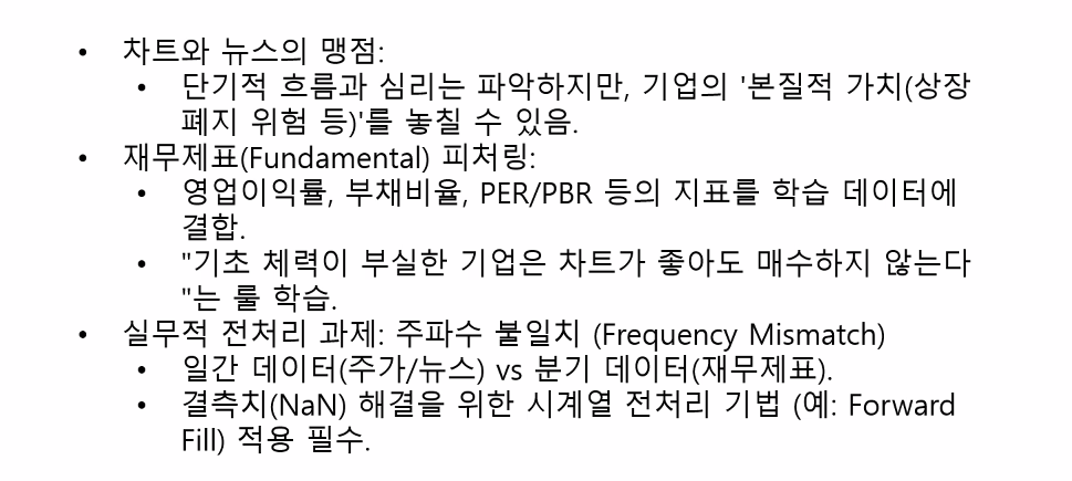
퀀트 트라이앵글 — 재무 데이터 결합

주식 데이터 실습

13. SK하이닉스 주가 예측 실습

데이터 수집 & 기술적 지표 생성

import yfinance as yf
import pandas as pd
import numpy as np

# SK하이닉스 최근 2년 데이터
hynix = yf.Ticker('000660.KS')
df    = hynix.history(period='2y')

df = df[['Close', 'Volume']]

# 20일 이동평균선
df['MA20'] = df['Close'].rolling(20).mean()

# 타겟 변수 — 내일 종가가 내일 20일 이평선보다 높은가?
df['target'] = (df['Close'].shift(-1) > df['MA20'].shift(-1)).astype(int)

df['target'].value_counts()

💡 shift(-1) — 데이터를 위로 1칸 이동 (내일 값을 오늘 행에 가져옴)
astype(int) — True/False → 1/0으로 변환
to_numeric() — 문자로 된 숫자를 수치형으로 변환 (변환 불가한 값은 NaN)

감성 점수 & DART 재무 데이터 추가

# 감성 점수 (실제로는 NLP로 생성, 여기서는 랜덤 대체)
df['MLP_Sentiment'] = np.random.uniform(-1, 1, len(df))

# DART API로 영업이익 데이터 수집
# !pip install OpenDartReader
import OpenDartReader
from datetime import datetime
import os
from dotenv import load_dotenv

load_dotenv()
api_key = os.getenv('api_key')

# 시차 정보 제거 (시계열 데이터 결합을 위해)
df.index = df.index.tz_localize(None)

dart         = OpenDartReader(api_key)
current_year = datetime.now().year
years        = [current_year - 2, current_year - 1, current_year]
report_codes = ['11013', '11012', '11014', '11011']   # 1Q, 2Q, 3Q, 연간

dart_data_list = []

for year in years:
    for code in report_codes:
        try:
            report = dart.finstate('000660', year, code)
            if report is not None:
                op_profit = report[
                    (report['fs_div'] == 'CFS') &
                    (report['account_nm'] == '영업이익')
                ]
                if not op_profit.empty:
                    val = int(op_profit['thstrm_amount'].values[0].replace(',', ''))

                    if   code == '11013': d = f"{year}-05-15"
                    elif code == '11012': d = f"{year}-08-14"
                    elif code == '11014': d = f"{year}-11-14"
                    else:                 d = f"{year+1}-03-31"

                    report_date = pd.to_datetime(d)
                    if report_date <= datetime.now():
                        dart_data_list.append({'Date': report_date, 'Operation_Profit': val})
        except:
            continue

dart_df = pd.DataFrame(dart_data_list)

# merge_asof — 날짜 기준 가장 가까운 이전 값으로 병합 (forward fill 효과)
df = pd.merge_asof(df, dart_df, left_index=True, right_on='Date', direction='backward')

기본 모델 & 클래스 가중치 모델 비교

from sklearn.ensemble import RandomForestClassifier
from sklearn.metrics import classification_report

x = df[['Volume', 'MA20', 'MLP_Sentiment', 'Operation_Profit']]
y = df['target']

# 시계열 데이터 분할 — 앞 80% Train / 뒤 20% Test (shuffle 금지)
split_idx = int(len(df) * 0.8)
X_train, X_test = x.iloc[:split_idx], x.iloc[split_idx:]
y_train, y_test = y.iloc[:split_idx], y.iloc[split_idx:]

# 기본 모델
model = RandomForestClassifier(random_state=42)
model.fit(X_train, y_train)
print(classification_report(y_test, model.predict(X_test)))

# 클래스 가중치 적용
model = RandomForestClassifier(random_state=42, class_weight='balanced_subsample')
model.fit(X_train, y_train)
print(classification_report(y_test, model.predict(X_test)))

파생 변수 추가 & 최종 모델

# 전일 대비 수익률
df['Return'] = df['Close'].pct_change()

# 거래량 변화율
df['Volume_change'] = df['Volume'].pct_change()

# 이격도 — 현재 주가가 20일 이평선에서 몇 % 떨어져있는가?
df['Dist_MA20'] = (df['Close'] - df['MA20']) / df['MA20']

df.dropna(inplace=True)

x = df[['MLP_Sentiment', 'Operation_Profit', 'Return', 'Volume_change', 'Dist_MA20']]
y = df['target']

split_idx = int(len(df) * 0.8)
X_train, X_test = x.iloc[:split_idx], x.iloc[split_idx:]
y_train, y_test = y.iloc[:split_idx], y.iloc[split_idx:]

model_final = RandomForestClassifier(random_state=42, class_weight='balanced_subsample')
model_final.fit(X_train, y_train)

print(classification_report(y_test, model_final.predict(X_test)))

⚠️ 시계열 데이터에서 train_test_split 주의
시계열 데이터는 shuffle=False 로 시간 순서를 유지해야 합니다.
train_test_split() 대신 인덱스 슬라이싱으로 직접 분할하는 것이 안전합니다.

📎 핵심 개념 요약

개념	설명
DBSCAN	밀도 기반 군집화 — k 지정 불필요, 이상치 자동 감지
`labels_ == -1`	DBSCAN 노이즈 데이터
`NearestNeighbors`	최근접 이웃 거리 계산 — 최적 eps 탐색에 활용
`np.diff()`	배열의 인접 원소 간 차이 계산
Elbow Point	그래프에서 기울기가 급변하는 지점 → 최적 eps
FDS	이상거래 탐지 시스템 — 재현율이 핵심 지표
Velocity	빈도/속도 기반 파생변수 — 사기 패턴 수치화
SHAP	전체 변수 기여도 분배 (게임 이론 기반)
LIME	개별 예측 국소적 설명
PDP	특정 변수 변화에 따른 예측 트렌드 파악
`shift(-1)`	데이터를 위로 1칸 이동 (내일 값 참조)
`pct_change()`	전일 대비 변화율 계산
`merge_asof()`	날짜 기준 가장 가까운 이전 값으로 병합
이격도	(현재 주가 - 이평선) / 이평선 × 100
미래 참조 오류	학습 시 미래 정보가 섞이는 치명적 오류
`tz_localize(None)`	시계열 인덱스의 시차 정보 제거
`class_weight='balanced_subsample'`	RandomForest에서 클래스 불균형 보정

syeom

공부 기록

이전 포스트

XGBoost & PCA & K-Means & t-SNE 실습 정리

다음 포스트

DBSCAN & 금융 데이터 분석 & 주식 데이터 실습 정리

멀티캠퍼스 데이터분석_11회차

📌 목차

DBSCAN

1. DBSCAN 이론 & 매개변수

동작 원리

주요 매개변수

algorithm 옵션

주요 속성

파라미터 튜닝 팁

2. DBSCAN 실습 — bodyPerformance 데이터

데이터 로드 & 전처리

NearestNeighbors로 최적 eps 탐색

DBSCAN 학습 & 검증

PCA 2차원 축소 후 군집 시각화

eps 값 변경 비교

금융 데이터 이론

3. 금융 데이터의 3대 특징

4. 이상거래 탐지(FDS) & 재현율

5. 실제 FDS 아키텍처 — 하이브리드 전략

6. FDS 피처 엔지니어링 — 벨로시티(Velocity)

7. 진화하는 사기 탐지 — 네트워크(Graph) 분석

8. XAI — AI의 속마음을 해부하다

금융 데이터 실습

9. 신용카드 사기 탐지 실습 — creditcard 데이터

데이터 로드 & EDA

시간대별 정상 vs 사기 거래 밀도 그래프

사기 결제 절대량 & 비율 시각화

모델 학습 & 불균형 처리 비교

SMOTE 적용 후 재학습

SHAP — 변수 기여도 시각화

LIME — 개별 예측 설명

PDP — 결제 시간대가 사기 판정에 미치는 영향

주식 데이터 이론

10. 시계열 데이터와 미래 참조 오류

11. 왜 이평선 기준 이진 분류인가?

12. 대안 데이터 — 감성 분석 & 재무 데이터 결합

NLP 감성 분석 파이프라인

NLP 스코어 + 정형 데이터 결합

퀀트 트라이앵글 — 재무 데이터 결합

주식 데이터 실습

13. SK하이닉스 주가 예측 실습

데이터 수집 & 기술적 지표 생성

감성 점수 & DART 재무 데이터 추가

기본 모델 & 클래스 가중치 모델 비교

파생 변수 추가 & 최종 모델

📎 핵심 개념 요약

XGBoost & PCA & K-Means & t-SNE 실습 정리

AARRR & 마케팅 데이터 분석 실습 & 딥러닝 이론 정리

0개의 댓글