[논문 Review] An image is worth 16x16 words: Transformers for image recognition at scale(ViT 논문)

[Paper] [Github]
Dosovitskiy, A., Beyer, L., Kolesnikov, A., Weissenborn, D., Zhai, X., Unterthiner, T., ... & Houlsby, N
ICRL 2021

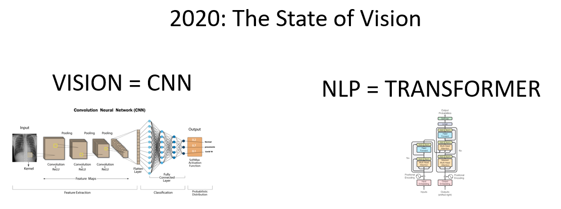Fig 1. The State of Vision

기존 Computer Vision 분야에서는 CNN 방법이 대다수였고 NLP 분야에서는 Transformer가 대세였다.
Vision 분야에서는 Transformer의 방법론을 사용할 수 없는데 그 이유는 224 x 224 이미지의 경우 50,176 pixels가 attention 방법을 적용하면 50k x 50k = 2.5B 연산량이 증폭되기 때문에 쓸 수 없었다.

그래서 저자들은 pixel 단위가 아닌 Patch 단위로 이미지를 넣어 Transformer 방법론을 사용 가능하게 만들었다.

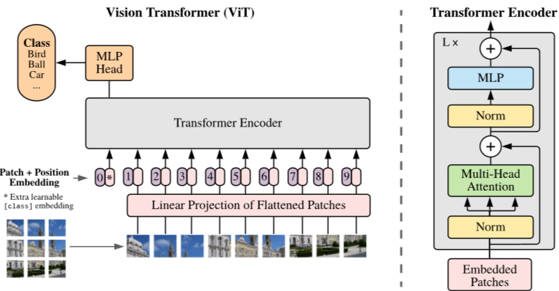
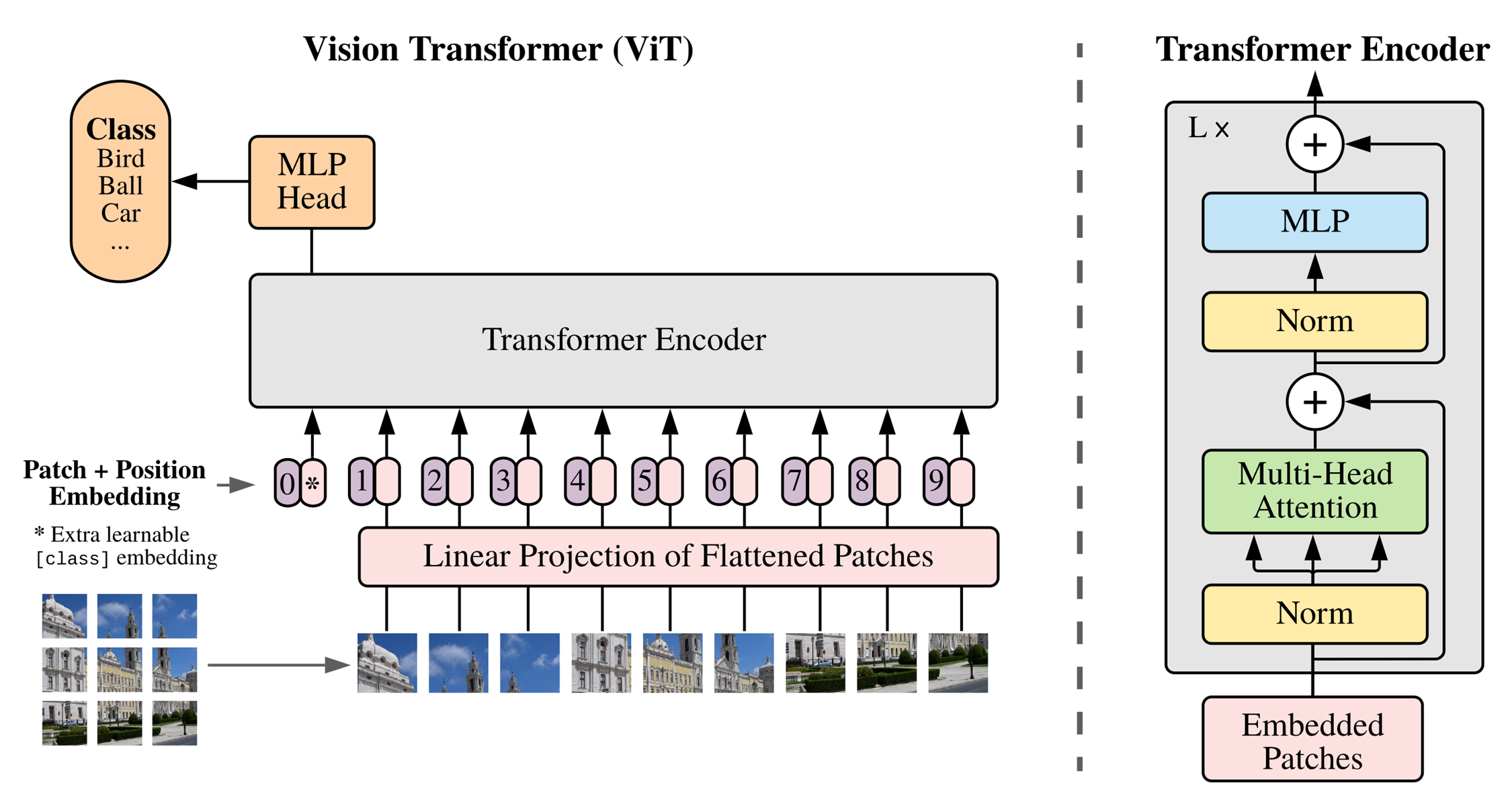Fig 2. ViT Architecture

위 그림은 ViT 논문의 파이프라인이다. 총 5단계로 구성이 되어있으며 각 단계별로 살펴보겠다.

1단계 : Image to Patches

• 일반적인 Transformer은 토큰 embedding에 대해 1차원의 sequence를 입력으로 받음
• 2차원의 이미지를 다루기 위해 이미지를 flatten된 2차원 패치의 sequence로 변환함
• 이미지 𝑥∈ℝ^(ℍ×𝕎×ℂ) 가 있을 때 이미지를 (P X P) 크기의 패치 𝑁=𝐻𝑊/𝑃^2 개로 분할하여 패치 sequence 𝑥_𝑝∈ℝ^(ℕ×(ℙ^𝟚⋅ℂ) ) 를 구축함

2단계 : Linear Projection of Flattened Patches

• Trainable linear projection을 통해 x_p의 각 patch를 flatten한 벡터를 D차원으로 변환한 후 이를 패치 임베딩으로 사용함

Equation 1. flatten the patches and map to D dimensions with a trainable linear projection

3단계 : Patch + Position Embedding

• ViT에서는 4가지 position embedding을 시도한 후 가장 효과가 좋은 1D position embedding을 ViT에 사용함
• Learnable class embedding과 patch embedding에 learnable postion embedding을 더함
• 처음 단계에 [CLS] 토큰을 추가해 토큰 전체를 대표함

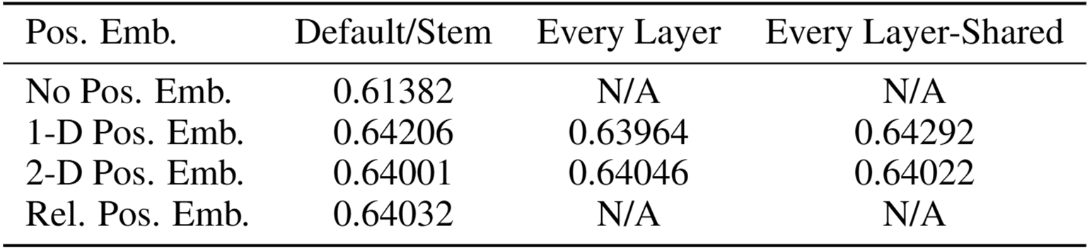Table 1: Results of the ablation study on positional embeddings with ViT-B/16 model evaluated on ImageNet 5-shot linear

4단계 : Transformer Encoder

• Vit는 Multi-head Self Attnetion(MSA)와 MLP blck으로 구성되어 있음
• MLP는 2개의 layer를 가지면 GELU activation function을 사용함
• 각 block의 앞에는 Layer Norm(LN)을 적용하고 각 block의 뒤에는 residual connection을 적용함
• embedding을 Transformer Encoder에 넣어서 output layer에서 class embedding에 대한 output인 image representation을 도출함

Equation 2. Transformer Encoder

5단계 : MLP Head

• MLP에 image representation을 input으로 넣어 이미지 class를 분류함

ViT는 아래와 같이 class와 이미지의 개수가 각각 다르 3개의 데이터셋을 기반으로 pre-train 되었다.
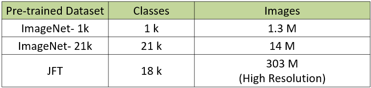Table 2: ViT Dataset

ViT는 아래와 같이 총 3개의 volume에 대해 실험을 진행했으며 다양한 패치 크기에 대해 실험을 진행했다.
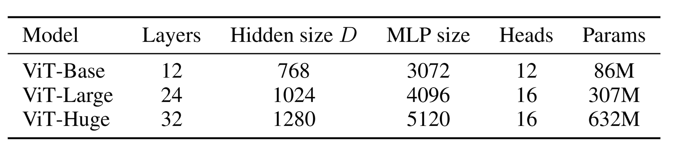Table 3. Details of Vision Transformer model variants

본 실험에서는 14 x 14 패치 크기를 사용한 ViT-Huge와 16 x 16 패치 크기를 사용한 ViT-Large의 성능을 baseline과 비교했다. (ViT-H/14 = ViT-Huge 모델에서 14 패치 크기를 사용했다는 뜻)

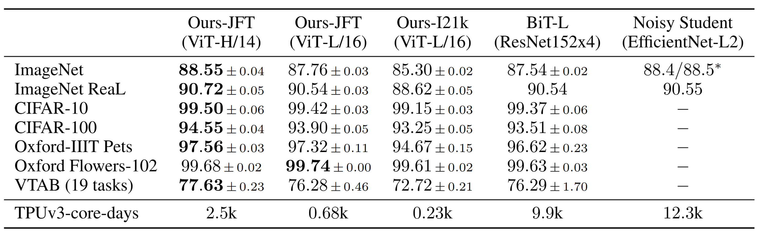Table 4. Comparison with state of the art on popular image classification benchmarks

본 논문은 19-task VTAB classification suite를 아래와 같이 3개의 그룹으로 나누어 추가 실험을 진행했는데 전체 데이터 뿐만 아니라 각 그룹에서도 ViT-H/14가 좋은 결과를 도출했다.
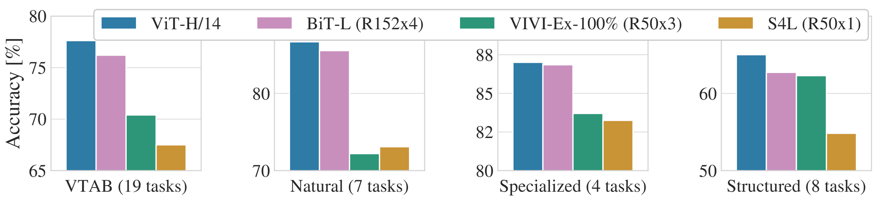Fig 3. Breakdown of VTAB performance in Natural, Specialized, and Structured task groups

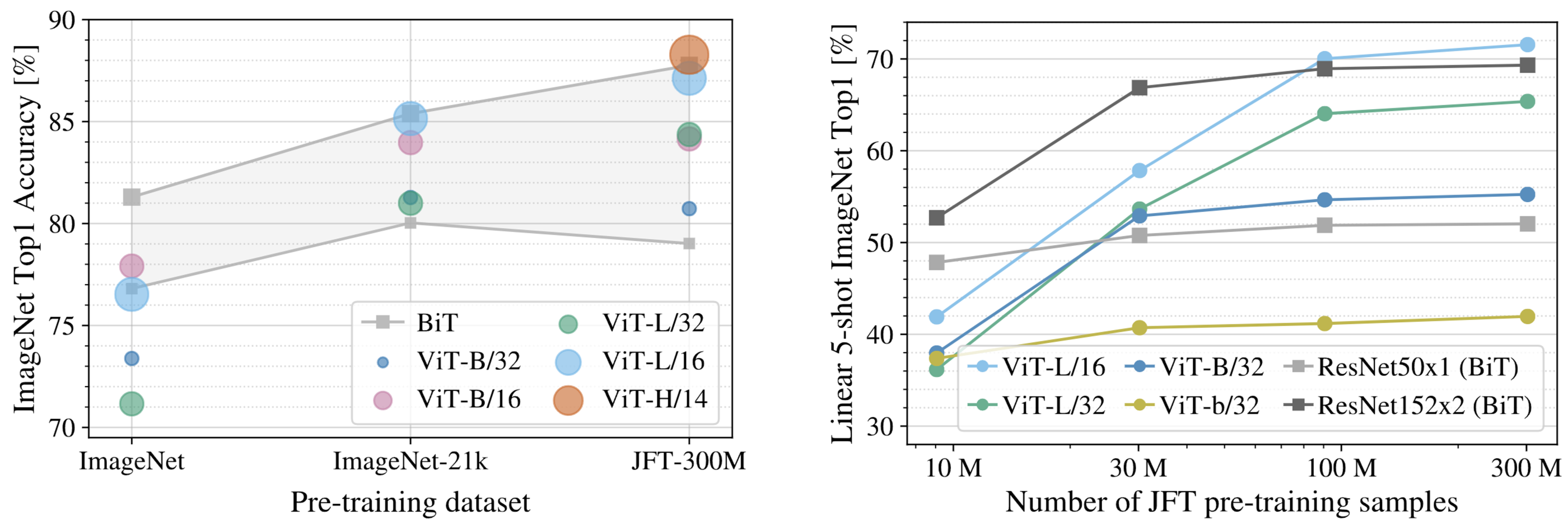Fig 4. Transfer to ImageNet. Whilelarge ViT models perform worse than BiTResNets (shaded area) when pre-trained onsmall datasets, they shine when pre-trained onlarger datasets. Similarly, larger ViT variantsovertake smaller ones as the dataset grows
Fig 5. Linear few-shot evaluation on Ima-geNet versus pre-training size. ResNets per-form better with smaller pre-training datasetsbut plateau sooner than ViT, which performsbetter with larger pre-training. ViT-b is ViT-Bwith all hidden dimensions halved.102 103

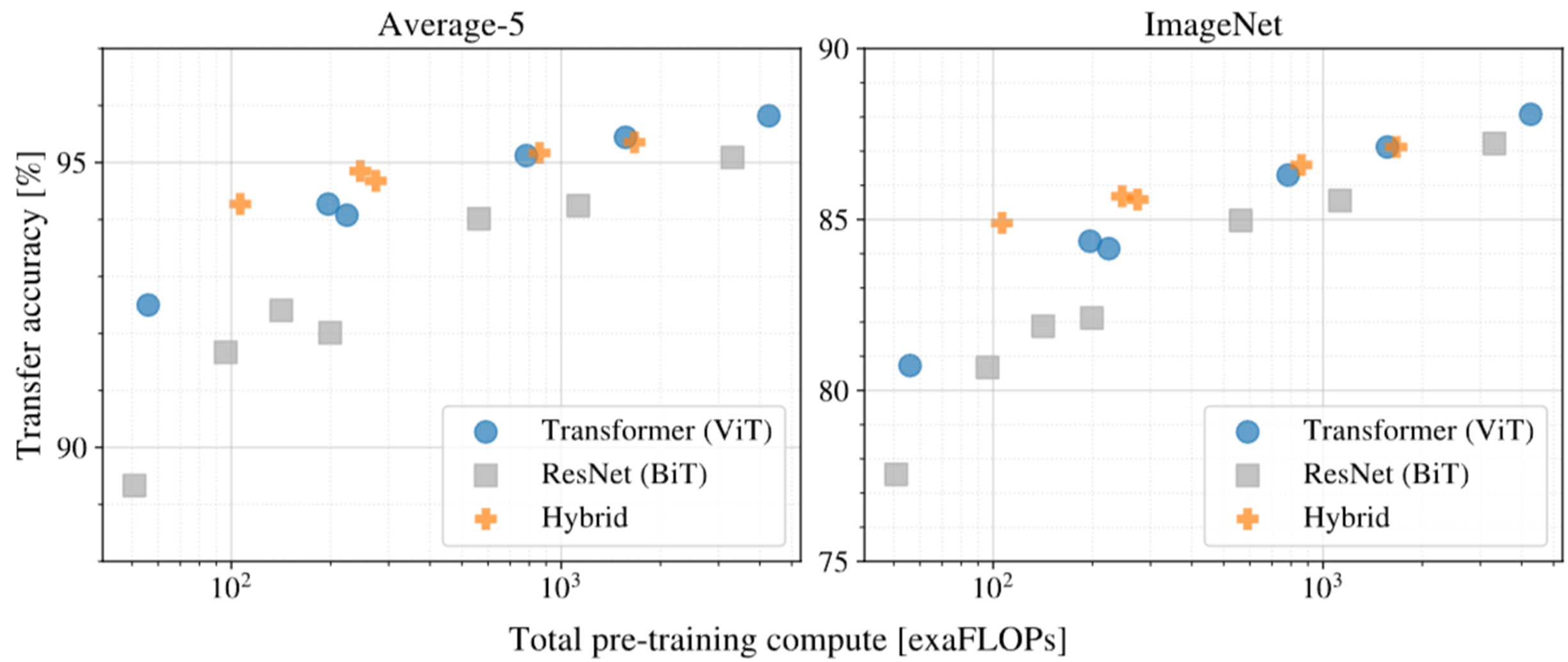Fig 6. Performance versus pre-training compute for different architectures: Vision Transformers, ResNets, and hybrids

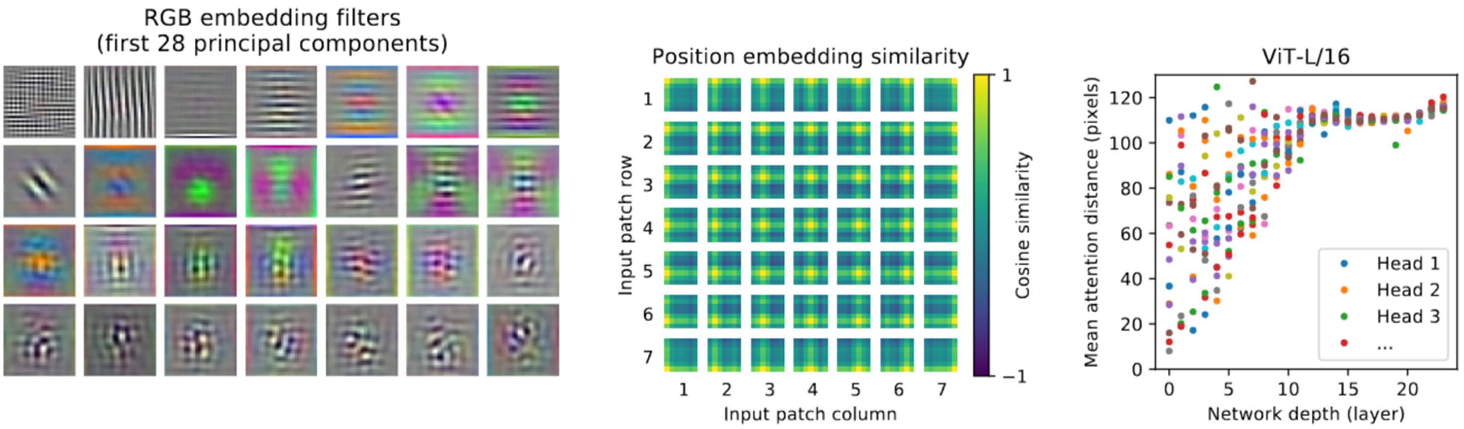Fig 7. Left: Filters of the initial linear embedding of RGB values of ViT-L/32. Center: Sim-ilarity of position embeddings of ViT-L/32. Tiles show the cosine similarity between the positionembedding of the patch with the indicated row and column and the position embeddings of all otherpatches. Right: Size of attended area by head and network depth. Each dot shows the mean attentiondistance across images for one of 16 heads at one layer. See Appendix D.7 for detail

ViT에서는 모델에 아래 두 가지 방법을 사용하여 inductive bias(새로운 데이터에 대해 예측을 할 떄 미리 가지고 있는 편향)의 주입을 시도함

• Patch extraction : cutting the image into pathes
• Resolution adjustment : adjusting the position embeddings for images of different resolutioin at fine-tuning

Future works로는 다음과 같다.

• ViT는 image classification에서만 좋기 때문에 detection과 segmentation인 다른 task에도 적용해봐야 함
• 정답 label이 없는 데이터에서는 학습이 가능하게 자체 지도 학습 기술(self-supervised learning)을 더 발전 시켜야 함
• 모델 크기를 더 늘리면 성능이 더 좋아질 것으로 예쌍