학습내용
NLP 기본개념
<용어정리>
토큰 : 단어, 형태소
corpus(말뭉치) : 특정한 목적을 가지고 수집한 텍스트 데이터
문장(Sentence) : 여러 개의 토큰으로 구성된 문자열. 기호로 구분
문서(Document) : 문장들의 집합
벡터화(vectorize) : 자연어를 컴퓨터가 이해할 수 있도록 벡터로 만들어주는 과정.
- count-based representation : 단어가 문서에 등장하는 횟수를 기반으로 벡터화, bag-of-words/TF-IDF
- distributed representation : 타겟 단어 주변에 있는 단어를 기반으로 벡터화, Word2Vec/GloVe/fastText
<NLP 사용>
- 자연어 이해(NLU)
- 분류 : 뉴스 기사 분류, 감성 분석
- 자연어 추론
- 기계 독해, 질의 응답
- 자연어 생성(NLG)
- 텍스트 생성 : 뉴스 기사 생성, 가사 생성
- NLU + NLG
- 기계 번역
- 요약 : 추출요약(NLU), 생성요약(NLG)
- 챗봇
- 기타
- text to speech
- speech to text
- image captioning
<텍스트 전처리>
- 내장 메서드 사용(replace 등)
- 정규표현식
- 불용어 처리
- 통계적 트리밍 : 코퍼스 내에서 너무 많거나, 너무 적은 토큰을 제거하는 방법
- stemming : 어간 추출, 어간이란 단어의 의미가 포함된 부분을 말하며 접사등이 제거된 상태이다.
- lemmatiztion : 표제어 추출, 기본 사전형 단어 형태인 Lemma(표제어)로 변환, 복수는 단수형으로 동사는 타동사로 변환
Tokenizing
문장에 포함된 구성요소들을 token화 시킴.
import spacy
from spacy.tokenizer import Tokenizer

nlp = spacy.load("en_core_web_sm")

tokenizer = Tokenizer(nlp.vocab)- tokenizer.pipe(text) : 인덱싱 가능 객체들을 인덱스 단위로 tokenize 해주는듯
- tokenizer(text) : tokenizing 해줌 [i.text for i in tokenizer(text)]를 통해 모든 token 문자열로 불러오기 가능
- nlp(text)를 통해서 tokenizing도 가능한데 결과가 tokenizer를 이용한 것과 조금 다름
Counter를 이용하여 bag of words 쉽게 구현가능
from collections import Counter

# Counter 객체는 리스트요소의 값과 요소의 갯수를 카운트 하여 저장하고 있습니다.
# 카운터 객체는 .update 메소드로 계속 업데이트 가능합니다.
word_counts = Counter()

df['tokens'].apply(lambda x: word_counts.update(x))

word_counts.most_common(10)
빈도가 높은 순서대로 rank 매겨주기
# 단어의 순위
# method='first': 같은 값의 경우 먼저나온 요소를 우선
wc['rank'] = wc['count'].rank(method='first', ascending=False)
각 토큰이 차지하는 정도 시각화, squarify 사용
#!pip install squarify
import squarify
import matplotlib.pyplot as plt

color=['viridis']

wc_top20 = wc[wc['rank'] <= 20]
squarify.plot(sizes=wc_top20['percent'], label=wc_top20['word'], alpha=0.6)
plt.axis('off')
plt.show()
불용어 처리
<불용어>
#확인
nlp.Defaults.stop_words

#불용어 없애기
tokens = []

#토큰에서 불용어 제거, 소문자화 하여 업데이트

for doc in tokenizer.pipe(df['reviews.text']):
    doc_tokens = []

    # A doc is a sequence of Token(<class 'spacy.tokens.doc.Doc'>)
    for token in doc:
        # 토큰이 불용어와 구두점이 아니면 저장
        if (token.is_stop == False) & (token.is_punct == False):
            doc_tokens.append(token.text.lower())

    tokens.append(doc_tokens)

df['tokens'] = tokens
df.tokens.head()
<불용어 커스터마이징>
STOP_WORDS = nlp.Defaults.stop_words.union(['batteries','I', 'amazon', 'i', 'Amazon', 'it', "it's", 'it.', 'the', 'this'])

tokens = []

for doc in tokenizer.pipe(df['reviews.text']):

    doc_tokens = []

    for token in doc:
        if token.text.lower() not in STOP_WORDS:
            doc_tokens.append(token.text.lower())

    tokens.append(doc_tokens)

df['tokens'] = tokens
stemming
어간 추출, 어간이란 단어의 의미가 포함된 부분을 말하며 접사등이 제거된 상태이다.
spacy에서는 stemming을 지원하지않으므로 nltk 사용
from nltk.stem import PorterStemmer

ps = PorterStemmer()

words = ["wolf", "wolves"]

for word in words:
	print(ps.stem(word))
lemmatization
표제어 추출, 기본 사전형 단어 형태인 Lemma(표제어)로 변환, 복수는 단수형으로 동사는 타동사로 변환
# Lemmatization 과정을 함수로 만들어 봅시다
def get_lemmas(text):

    lemmas = []

    doc = nlp(text)

    for token in doc:
        if ((token.is_stop == False) and (token.is_punct == False)) and (token.pos_ != 'PRON'): #token.pos_ : 품사를 나타냄, PRON은 대명사
            lemmas.append(token.lemma_)

    return lemmas
Bag of Words
<특징>
문서를 구성하고 있는 모든 단어들을 가방에 집어넣은 후 하나씩 꺼내며 각 단어의 개수를 세어주는 개념. 이를 통해 문서를 벡터화 할 수 있다.
벡터화된 문서는 단어의 종류만큼 feature를 가지며, 각 단어의 개수를 해당 feature의 값으로 설정한다.
<단점>
-sparsity
-frequent words has more power
-ignoring word orders
-out of vocabulary
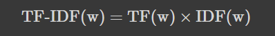
TF-IDF(Term frequency-Inverse document frequency)
<구현>
# 모듈에서 사용할 라이브러리와 spacy 모델을 불러옵니다.
import pandas as pd
import seaborn as sns
import matplotlib.pyplot as plt

from sklearn.feature_extraction.text import CountVectorizer, TfidfVectorizer
from sklearn.metrics.pairwise import cosine_similarity
from sklearn.neighbors import NearestNeighbors
from sklearn.decomposition import PCA

import spacy
nlp = spacy.load("en_core_web_sm")
from sklearn.feature_extraction.text import CountVectorizer
## stop_words = 'english' 영어에 해당하는 불용어 처리를 합니다.
## max_features=n, 빈도 순서대로 top n 단어만 사용합니다.
vect = CountVectorizer(stop_words='english'
, max_features=10000)
# fit & transform
dtm = vect.fit_transform(data)
dtm = pd.DataFrame(dtm.todense(), columns=vect.get_feature_names())
dtm.shapeTF-IDF(Term Frequency - Inver Documnet Frequency)
각 token마다 문장에서의 중요도를 계산하여 벡터화 시키는 방법이다.
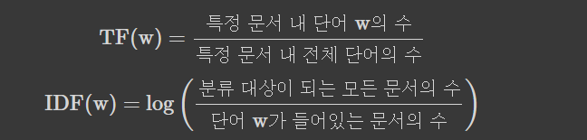
token의 중요도는 코퍼스(모든 문서)에 token이 많이 사용될수록 중요한 token이라 판단하여 가중치(TF)를, 많은 문서에 사용되면 사용될수록 문서를 구분짓는데 의미가 없는 token이라 판단하여 패널티(IDF)를 주는 개념이다.
<계산 수식>
<구현>
# TF-IDF vectorizer. 테이블을 작게 만들기 위해 max_features=15로 제한하였습니다.
tfidf = TfidfVectorizer(stop_words='english', max_features=15)

# Fit 후 dtm을 만듭니다.(문서, 단어마다 tf-idf 값을 계산합니다)
dtm = tfidf.fit_transform(text)

dtm = pd.DataFrame(dtm.todense(), columns=tfidf.get_feature_names())
dtm


#파라미터 튜닝
# spacy tokenizer 함수
def tokenize(document):

    doc = nlp(document)
    # punctuations: !"#$%&'()*+,-./:;<=>?@[\]^_`{|}~
    return [token.lemma_.strip() for token in doc if (token.is_stop != True) and (token.is_punct != True) and (token.is_alpha == True)]

# ngram_range = (min_n, max_n), min_n 개~ max_n 개를 갖는 n-gram(n개의 연속적인 토큰)을 토큰으로 사용합니다.
# min_df = n, 최소 n개의 문서에 나타나는 토큰만 사용합니다
# max_df = .7, 70% 이상 문서에 나타나는 토큰은 제거합니다
tfidf = TfidfVectorizer(stop_words='english'
                        ,tokenizer=tokenize
                        ,ngram_range=(1,2)
                        ,max_df=.7
                        ,min_df=3
#                         ,max_features = 4000
                       )

dtm = tfidf.fit_transform(data)
dtm = pd.DataFrame(dtm.todense(), columns=tfidf.get_feature_names())
dtm.head()- max_df와 min_df를 잘못 설정하면 에러가 발생. max_df * 문서수 < min_df 인 경우
NearestNeighbor(KNN)
각 문서를 벡터화했으니 문서끼리의 유사도를 측정하여보자.
사용하는 알고리즘은 KNN으로, 쿼리와 가장 가까운 상위 K개의 근접한 데이터를 찾아서 K개 데이터의 유사성을 기반으로 점을 추정하거나 분류하는 예측 분석에 사용된다.
<구현>
from sklearn.neighbors import NearestNeighbors

# dtm을 사용히 NN 모델을 학습시킵니다. (디폴트)최근접 5 이웃.
nn = NearestNeighbors(n_neighbors=5, algorithm='kd_tree')
nn.fit(dtm)
<377번째 문서와 가장 유사한 5개의 문서 찾기>
nn.kneighbors([dtm.iloc[377]])<새로운 문서와 가장 유사한 5개의 문서 찾기>
new = tfidf.transform(cnn_tech_article)
nn.kneighbors(new.todense())