=== Congestion Control ===
라우터에 들어오는 패킷이 많아서 패킷 드랍이 발생하는 상황
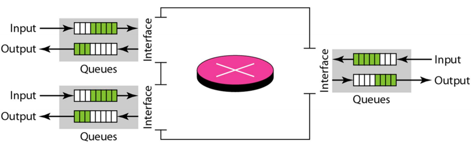
1. Congestion
- Even if receiver’s buffer is empty, segments may be dropped at the routers
- If input speed is faster than output speed at the router, the buffer fills up -> delay increases : 라우터의 input speed가 output speed보다 빨라서 버퍼가 가득차고 딜레이가 늘어나게 된다.
- Finally the buffer overflows -> PACKET DROP : 결국에는 패킷을 드랍하게 된다.
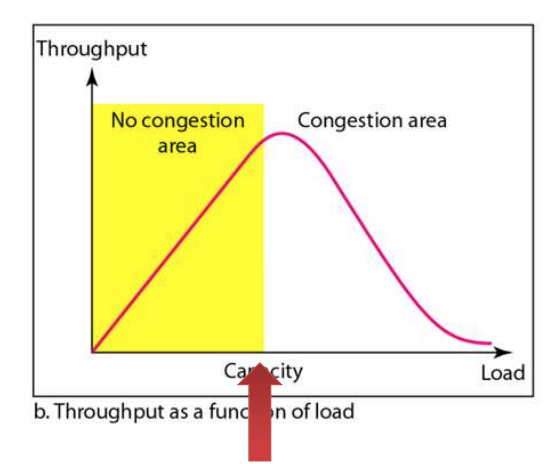
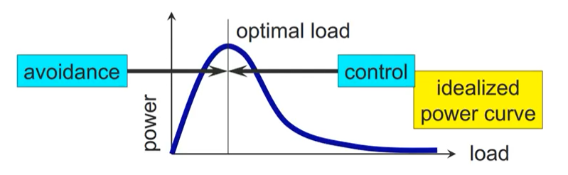
load(전달되는 트래픽의 양), delay, throughput(1초에 전달가능 데이터)
load가 많아질수록 딜레이가 급하게 늘어나서 무한하게 간다(buffer free)
capacity : 네트워크가 감당할 수 있는 양
throughput은 일정수준 이상가면 전달되는 데이터 양이 줄어들게 된다. packet drop으로 계속 패킷이 재전송이 되다보니 중복데이터가 점차많아지게 된다.
- Delay increases as the load becomes higher. Delay becomes infinity when the load reaches capacity.
- When the load is high, throughput begins to drop
(요약)
네트워크가 감당못하는 수준으로 보내는 것을 컨트롤 하는 것이다.
네트워크에 congestion이 발생했다고 판단되면 속도를 줄여야 한다.
congestion은 어떻게 판단하는가? 네트워크의 코어는 아무것도 해주지 않는다. forwarding만 해준다. 그럼 end host에서 congestion을 점검해야한다.
패킷이 잃어버렸는지 딜레이가 발생했는지를 바탕으로 속도를 제어해야한다.
-
load(전달되는 트래픽의 양), delay, throughput(1초에 전달가능 데이터)
-
load가 많아질수록 딜레이가 급하게 늘어나서 무한하게 간다(buffer free)
-
capacity : 네트워크가 감당할 수 있는 양
-
throughput은 일정수준 이상가면 전달되는 데이터 양이 줄어들게 된다. packet drop으로 계속 패킷이 재전송이 되다보니 중복데이터가 점차많아지게 된다.
Congestion Control: Goal
capacity : 시시각각 바뀔수가 있는 값이다. sender 입장에서 어느정도의 속도까지 보내면 congestion이 발생하지 않으면서도 최대한 많은 양을 보낼 수 있는지에 대한 값이다.
- Sliding window size -> Load
- Control load in order to achieve best throughput
Congestion Control: Method
- Routers cannot give feedback : 라우터가 feedback을 주지 않기때문에 직접해보는 수밖에 없다.
- TCP congestion control approach: BY EXPERIENCE
- No congestion -> Increase CWND (Congestion Window)
- Congestion -> Decrease CWND
- Sign of congestion = LOST PACKET : congestion이 일어난걸 확인하는 방법은 패킷 LOST가 발생했다는 것을 확인하는 방법뿐이다.
- Assumption: packet loss is unlikely to
occur by other means : 가정으로 다른 방식으로 packet loss가 발생하지 않는다 생각한다. - This assumption may not hold in wireless LANs (Wi-Fi) : 하지만 요즘에는 Wi-Fi로 packet loss가 발생하는 경우가 생기기도 한다.
- Assumption: packet loss is unlikely to
Congestion Control: Basics
- Controlled variable: CWND
- Sliding window size: min(RWND, CWND)
- Unit: MSS (Maximum Segment Size) : 기본단위로 사용한다.
- Initial CWND: 1 MSS : 한 세그먼트를 처음 보낼때 1MSS만큼 보내고 이후에 MSS를 늘린다.
- Initial Phase: SLOW START : 시작은 SLOW START Phase로 시작한다.
(요약)
AIMD 방식
-
End Point에서 RTT 마다 cwnd의 MSS(Massive Segment Size)를 1씩 증가하도록 설정되어 있다.
(보통 1500byte 정도) -
loss가 발견되면 cwnd를 절반으로 줄인다.
-
sender limits transmission
LastByteSent - LastByteAcked <= cwnd
대충 노락색 부분이 cwnd보다는 작아야한다는 것이니 당연한것이다.
Slow Start Phase
- For each segment ACKed, increase CWND by 1 MSS : 처음에는 1 MSS만 보낸다. 그리고 ACK온 것을 보고 CWND를 늘린다.
- CWND = CWND + 1 (MSS) : ACK마다 증가시키기 때문에 굉장히 빠르게 증가한다.
- CWND increases EXPONENTIALLY -> fast increase : 기하급수적으로 증가하게 된다.
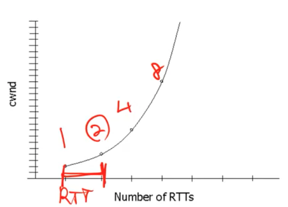

- For each RTT (Round-Trip Time), CWND doubles
- exponential increase
- Sending speed increases with CWND
- At some point, congestion will occur inevitably -> packet drop occurs : 언젠가는 congestion이 발생하게 된다. 그때 패킷이 drop된다.
- When a packet is dropped, the corresponding ACK will not come to the sender : 패킷이 drop되면 패킷에 대한 ACK은 전달되지 않는다.
(요약)
Fast Retransmission(TCP RENO)
- CWND = CWND + 1 (MSS) : ACK마다 증가시키기 때문에 굉장히 빠르게 증가한다.
지수적으로 증가한다. - 패킷이 drop되면 cwnd를 1로 바꾸어버린다.
- 드랍되고 다시 지수적으로 증가하지만 일정 threshold 부터는 선형적으로 증가한다.
- ACK가 3개 도착하면 그거역시 loss 로 판단한다. 이때는 1로 가지않고 1/2로 줄인후 선형저으로 증가한다. <-> TCP Tahoe는 그냥 1로 바꾼다.
TCP Tahoe는 이때 ssthresh를 마지막 최대치의 절반으로 바꾼다.
TCP Reno는 그냥 절반으로 줄이고 선형적으로 증가시킨다.
Timeout
- For each TCP segment, the sender keeps a timer : 각 TCP 세그먼트마다 timer가 존재한다.
- If ACK is not received for a certain duration of time, a TIMEOUT occurs : timeout이 발생가혐 해당 세그먼트는 lost 되었다고 판단하고 패킷을 재전송하게 된다.
- When timeout occurs, the segment is considered
LOST- The sender retransmits the segment
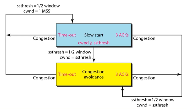
Slow Start and Timeout
- When a timeout occurs, : Timeout이 발생시
- SSThresh is set to CWND / 2 : 발생시의 CWND값의 반을 SSThresh 변수에 저장한다.
- SSThresh: Slow-Start Threshold
- CWND becomes 1 : CWND 를 1로 맞추고 Slow Start를 재시작하게 된다.
- Restart the Slow Start phase
Slow Start and SSThresh
- After timeout, CWND will start to increase again
- When CWND reaches SSThresh, the Slow Start phase ends : SSThresh까지 가면 Slow Start phase에서 Congestion avoidance phase로 바뀌게 된다.
- Sender enters the CONGESTION AVOIDANCE phase
(요약)
Congestion Avoidance Phase
-
For each RTT, CWND is increased by 1 MSS : RTT 마다 MSS가 1칸만 증가하도록 설정되어 있다.
- RTT: Round Trip Time
-
CWND += MSS * (MSS / CWND) : 갯수로 나누어서 1만 증가되도록 공식을 만든다.
-
Additive Increase
-
Congestion avoidance phase continues until a segment is lost : 다음 congestion이 발생할때까지 이것을 반복한다.
-
Slow Start: exponential increase
-
Congestion Avoidance: additive increase
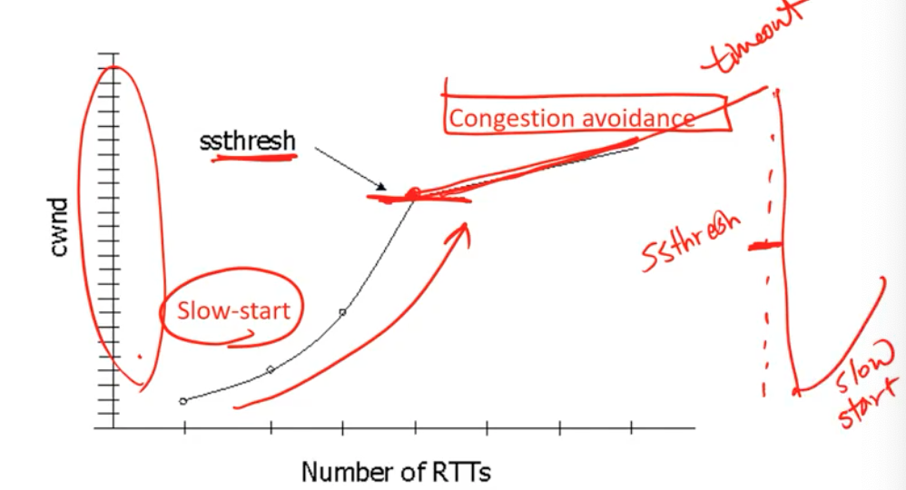
선형적으로 증가하는 부분을 Congestion avoidance라고 부른다.
Basic CWND behavior
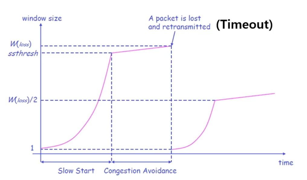
정리하면 위와 같은 형태로 작동하게 된다.
2. Timeout 1
- Sender sends a segment and wait for its ACK for a
duration of time (RTO: Retransmission TimeOut) : RTO의 값을 적절하게 설정해야 한다. - If ACK arrives, the timer is removed : ACK이 오면 timer 꺼주기
- If ACK does not arrive until timer expires, a TIMEOUT is occurred and the segment is retransmitted : timer이 만료되면 TIMEOUT과 함께 세그먼트를 재전송하게 한다.
Retransmission Timeout
- How long should the sender wait?
- If RTO is too short : RTO가 너무 짧으면 세그먼트가 loss가 없는데도 재전송하낟.
- timeout can occur even when the segment is not lost
- If RTO is too long
- When the segment is lost, the sender wastes too much time before retransmitting
- WHAT IS THE PROPER RTO?
Proper RTO
- Proper RTO: RTT (Round Trip Time) + margin
- margin needed to handle RTT variations
- TCP is an end-to-end protocol, so it is not easy to
know the RTT : RTT계산이 쉽지가 않다. 라우터 거칠때마다 달라진다. - RTT can vary over time
- Depending on status of intermediate routers
- HOW SHOULD WE ESTIMATE RTT?
- WHAT IS THE PROPER MARGIN?
RTT Estimation
- Original algorithm
- Measure RTT by sending data and receiving ACK
- measured RTT is called “SampleRTT”
- Compute “EstimatedRTT” by exponential averaging
- EstimatedRTT = a x EstimatedRTT + (1-a) sampleRTT : 앞에서 나온건데 기존값과 갔다온 RTT값으로 계산한다.(a = 0.875를 보통 사용한다)
- RTO = 2 x EstimatedRTT (마진은 그냥 2배를 준다)
- To add margin, we use twice the EstimatedRTT

- To add margin, we use twice the EstimatedRTT
- Measure RTT by sending data and receiving ACK
3. Timeout 2
-
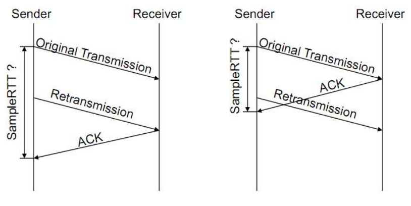
Original algorithm: problem
- If a segment is retransmitted and an ACK is received, we cannot know if the ACK is for the original segment or the retransmitted segment : 그럼 우리가 측정한 RTT값이 origin에서 보내진건지 retransmitted segment에서 보내진건지 알 수 없음
- can screw up RTT calculation
- can screw up RTT calculation
- If a segment is retransmitted and an ACK is received, we cannot know if the ACK is for the original segment or the retransmitted segment : 그럼 우리가 측정한 RTT값이 origin에서 보내진건지 retransmitted segment에서 보내진건지 알 수 없음
-
Karn/Partridge algorithm
- If a segment is retransmitted, the ACK for the segment is not used as SampleRTT : 재전송시에 오는 ACK는 SampleRTT에 포함시키지 않겠다.
- Exponential backoff
- If timeout occurs, RTO <- 2 x RTO : timeout이 발생시 기존의 RTO값을 두배로 해준다.
-
Why exponential backoff?
- If delay suddenly increases, all segments will be
retransmitted, and the timeout will not be updated : 딜레이가 갑자기 증가하면. 내가 원래 설정했던 값에서 계속해서 timeout이 발생할 수 있다. 여기에서 재전송한것에 대해서는 SampleRTT에 포함시키지 않겠다고 했다. 어느순간부터 내가 패킷이 계속 delay가 발생하여 drop이 되면 RTO를 갱신할 시간이 없다. 그래서 한 번이라도 RTO가 발생하면 두배로 만들겠다.
- If delay suddenly increases, all segments will be
-
Jacobson/Karels algorithm
- considers RTT variation
- If variation is small, RTO can be tight (small margin) : RTT의 variation이 작으면 RTO가 두배까지 될필요없다.
- If variation is large, RTO should be large (large margin) : RTT가 크면 RTO는 두배이상이 되어야 한다.
- Difference = SampleRTT – EstimatedRTT
- EstimatedRTT = EstimatedRTT + (δ x Difference)
- Deviation = Deviation + δ(|Difference| - Deviation)
- δ is a value between 0 and 1 (typically 0.25)
- RTO = EstimatedRTT + 4 x Deviatio
- considers RTT variation
=== Fast Retransmission and Fast Recovery ===
1. Fast Retransmission
-
When a segment is lost, it is known to sender when a
timeout occurs : 세그먼트 lost가 생기면 timeout이 생기었다는 뜻이다. -
However, it takes a long time before timeout occurs : timeout까지는 시간낭비가 존재한다.
- Waste of time
-
Fast Retransmission provides a way to quickly detect
a segment loss and retransmit the segment : 더 빠르게 segment loss를 확이나는 것이 Fast Retransmission이다. -
Duplicate ACK : 중복 ACK를 보고 판단하겠다.
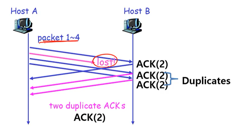
ACK(2)라는 것은 2번째 segment를 보내달라는 이야기로 중복이 발생했다. -
Three duplicate ACKs for a segment : 3개의 duplicate ACK이 왔다면
-> The segment is considered lost : 2번 segmet가 lost되었다고 판단
-> Retransmit the segment : segment 재전송하겠다. -
Why THREE?
- Out-of-order delivery possible at the IP layer : network 레이어에서 전송시 Out-of-order가 발생할 수 있다.
- Thus, a single duplicate ACK may not mean segment loss : 2개의 ACK 만으로 판단하는 것은 loss라고 하기는 힘들다.
- Three duplicate ACKs may be generated without segment loss, but that is unlikely to happen : 하지만 3개부터는 loss가 아닐 수 없다.
(요약)
sender 가 중복되는 ACK을 3번 받으면 다시보내겠다.
unacked segment with smallest seq를 다시보낸다.
위의 이미지와 같이 TCP 연결상에 중간에 하나가 lost되면 세그먼트의 첫번째를 ACK으로 요청하기 떄문에 중보되는 ACK이 발생할 수 밖에 없다.
Indication of a Segment Loss
indication은 두개가 되었다.
-
Timeout
-
Three duplicate ACKs
-
Slow Start +
Congestion Avoidance +
Fast Retransmission =
TCP Tahoe(1988)
Fast Recovery
-
When a segment loss is detected, the CWND is reset to 1 -> Too abrupt reduction in sending speed : 어떤 segment loss가 발생시 CWND는 1로 셋팅한다.
-
When segment loss is detected by 3 dup ACKs, do not go back to slow start, but restart from the congestion avoidance phase : 만약 3개의 중복 ACK에 의해 segment loss가 되면 congestion avoidance에서 시작하자
-
SSThresh <- CWND / 2 : 절반으로 줄이고 다시 시작하자
-
CWND <- SSThresh
-
TCP Tahoe + Fast Recovery -> TCP Reno
TCP Congestion control
TCP Reno의 작동방식 요약
- Timeout -> Slow-start
- Fast retransmission -> Congestion avoidance
CWND dynamic
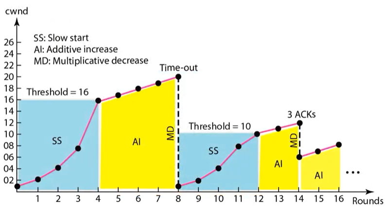
위의 모델을 그대로 따르면 위와 같은 그래프가 생기게 된다.
TCP CUBIC (2006)
- Adopted as the default TCP congestion control algorithm in Linux
- Designed for "long, fat" networks : 딜레이도 길고 bandwidth도 큰 네트워크, TCP CUBIC은 이런 long fat network에서 작동하기 위해 제작된 congestion control algorithm이다.
- end-to-end path has large delay and large bandwidth
- TCP CUBIC: approach
- congestion window adjusted at regular intervals, based on the amount of time that has elapsed since the last congestion event (the arrival of a duplicate ACK), rather than only when ACKs arrive (the latter being a function of RTT) : congestion window를 조정하는게 ACK이 오면 조정한다. 네트워크에 여러 connection이 있어서 RTT가 짧은 connection은 ACK이 빨리와서 조절하기 쉬운 반면 RTT가 긴건 조절하기 어렵다.
1.그래서 어느정도 시간안에 congestion이 없었으면 CWND를 늘리겠다.
- CUBIC function을 이용한다.
- use of a cubic function to adjust the congestion window
- Wmax: maximum congestion window size achieved just before the last congestion event : 저번에 congestion이 발생했을때 CWND 사이즈이다.
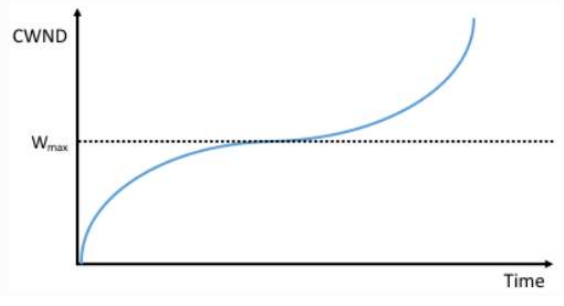
- Wmax: maximum congestion window size achieved just before the last congestion event : 저번에 congestion이 발생했을때 CWND 사이즈이다.
- congestion window adjusted at regular intervals, based on the amount of time that has elapsed since the last congestion event (the arrival of a duplicate ACK), rather than only when ACKs arrive (the latter being a function of RTT) : congestion window를 조정하는게 ACK이 오면 조정한다. 네트워크에 여러 connection이 있어서 RTT가 짧은 connection은 ACK이 빨리와서 조절하기 쉬운 반면 RTT가 긴건 조절하기 어렵다.
2. Congestion Avoidance
congestion control과 상반되는 개념
-
Congestion control: when congestion occurs, do
something to recover : congestion이 발생전에는 계속 늘리다 나중에 줄임 -
Congestion avoidance: avoid congestion before it
occurs : congestion이 발생전에 피할 수 있는 방법 찾기
-
Router-based congestion avoidance
- RED (Random Early Detection)
-
Source-based congestion avoidance
- TCP Vegas
Random Early Detection
- If the router is “almost” full, it starts to drop packets
randomly : 라우터가 거의 full인 상태라면, 패킷을 랜덤하게 drop하겠다. - TCP source reduces sending speed due to packet drop : TCP가 패킷 loss가 있었으니 sending speed를 조절한다.
이렇게 하는 이유는 잘못하면 라우터가 모든 패킷을 드랍할 수 있어서 미리 드랍하는 것이다.
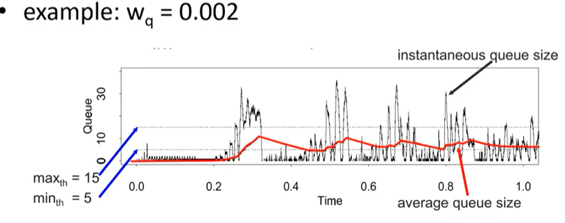
- Compute average queue length (AvgLen)
- AvgLen = (1-Weight)
*AvgLen + Weight*SampleLen : 계속해서 패킷의 갯수를(sampleLen) 계산하면서 Avgen을 업데이트한다. - 0 < weight < 1
- Typically, “weight” is a small value (e.g. 0.002)
- SampleLen: the queue length when a packet arrives(queue length를 패킷이 올때마다 측정을 해서 avglen 업데이트)
- AvgLen = (1-Weight)
- if AvgLen ≤ MinThreshold
- insert packet into the queue
- if MinThreshold < AvgLen < MaxThreshold
- probabilistically drop packet (based on drop probability p) : 사이에 있으면 p에 의해서 드랍시킨다.
- if MaxThreshold ≤ AvgLen
- drop packet
- computing average queue length: low-pass filter

TCP Vegas
- A variation of TCP
- uses congestion avoidance instead of congestion control
- detection congestion before packet is dropped
- if throughput does not increase much as congestion window is increased, it indicates that the network is near congestion : congestion window가 커짐에도 Throughput이 증가하지 않는 것을 감지한다.
- If there is no congestion, the throughput should be
as expected- ExpectedRate: congestion window / baseRTT : 안막히는 상황에서 이정도가 나오겠다는 것을 ExpectedRate로 한다.
- baseRTT: minimum measured RTT : 측정된 RTT중 가장 작은 것을 base RTT로 삼는다.
- Measure actual throughput
- Mark a certain packet : 어떤 패킷에 mark
- count the number of bytes sent until the ACK for the marked packet arrives. -> ActualRate : Mark한 패킷이 올때까지 몇 byte를 보냈는지 확인
- Diff = ExpectedRate – ActualRate
- if Diff < a : congestion이 아니기 때문에 늘린다.
- Increase CWND linearly
- if Diff > b : congestion에 가까우니 줄인다.
- Decrease CWND linearly
- else
- Leave CWND unchanged
- decide whether CWND should be increased or decreased, based on comparison between expected rate and actual rate
Additional Topic: QUIC
- HTTP/3 uses QUIC instead of TCP
- QUIC is based on UDP : UDP위에 기능을 언진것
- reliability and flow control built at the level of QUIC : reliability와 flow control을 올린것
- QUIC: characteristics compared to TCP : TCP 문제점을 완화
- greatly reduce overhead during connection setup : connection setup의 overhead 줄이기
- makes exchange of setup keys and supported protocols part of the initial handshake process : initial handshake에서 한꺼번에 해버려서 메세지가 오고가는 횟수를 줄여서 딜레이를 줄였다.
- remove the need to send additional packets for TLS (transport layer security)
- avoid head-of-line-blocking when packet is lost : 어떤 패킷 loss가 발생하면 다른 패킷들이 먼저갈 수 있도록한다.
- In TCP, all the following packets must wait until the packet is recovered
- In QUIC, other data can be freely processed
- greatly reduce overhead during connection setup : connection setup의 overhead 줄이기