ViSD-Boost (ICCV 2025)

Treeboy·2026년 1월 17일

CVPR준비

목록 보기

13/14

바로 이전에 CT-GLIP, fVLM 을 리뷰했었는데, 와 얘네들 또 똑같은거 우려먹어서 ICCV 에 냈다 ㅋㅋ. fVLM 에서는 그냥 pooling 방법 바꾸고 false negative 만 조금 정리했는데, 이번에는 anomaly detection 한스쿱을 넣어서 논문을 냈다. 얼렁 살펴보자.

Methods

Title: Boosting Vision Semantic Density with Anatomy Normality Modeling in Medical Vision-language Pre-training

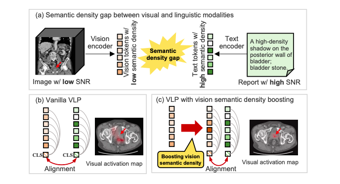
Semantic density: concentration of diagnostic-related signals conveyed within the representation of medical images. 만약 영상에서 병이 아주 국소적으로 발현한다면, low visual semantic density 라고 할 수 있겠다. 반면에, 영상 판독문에서는 병을 바로 언급하기 때문에 rich diagnostic-related semantics 가 존재한다. 이 두 modality 를 align 할 때 semantic density 의 gap 이 존재한다는 것이 핵심 발견이다. (아래 그림)

이걸 어떻게 해결하냐? Two key steps 를 제안한다.

(1) Enhancing vision semantics

특정 장기를 normal / abnormal 로 구분한다. 어떻게 하냐고? Qwen 써서 판독문을 정리한다. 목적은 normal sample 이 모여있는 embedding space 를 만들고, abnormal samples 는 normal samples 와 구분될 뿐 만 아니라 서로 distinct 하도록 만든다 (병이 생긴것도 제각각이기 때문이다).

이 단계는 vision only 로 진행하며, 둘 다 normal 이면 당기고, 둘 중 하나라도 abnormal 이면 밀어낸다.

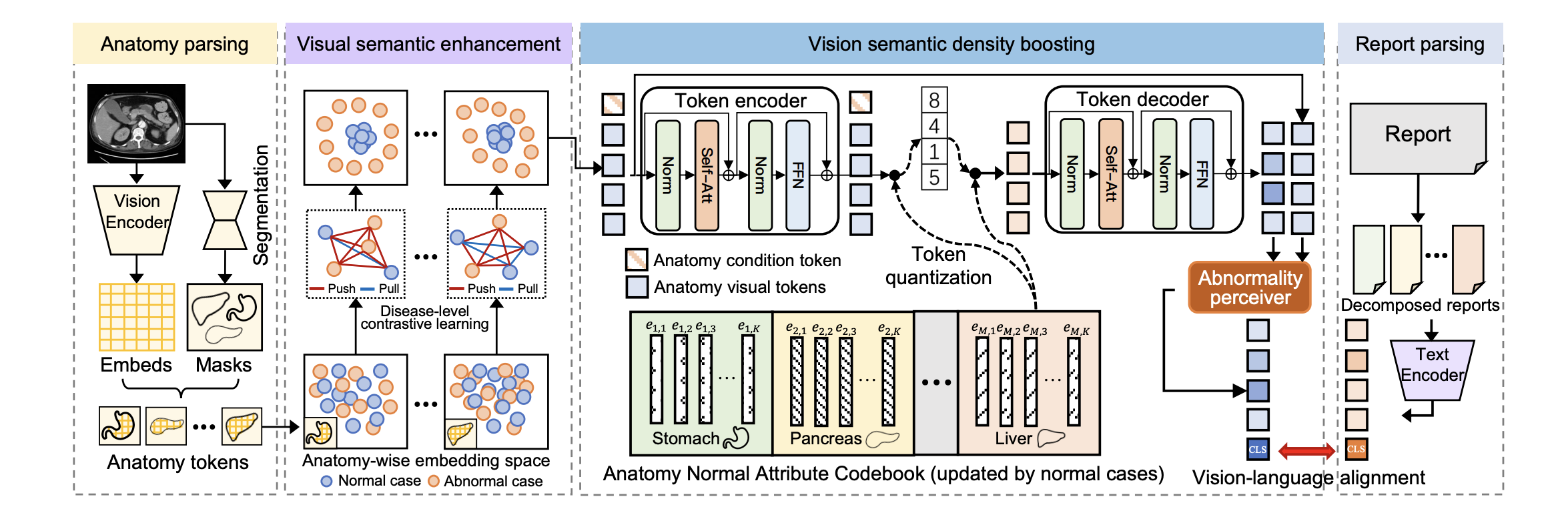
한가지 더. $Q^I_{i,j}$ 는 query token 이랑 organ 내의 patch ( $X^I_{i,j}$ ) 랑 attention 때려서 update 한건데, query 가 그냥 의미없이 무지성으로 $X^I_{i,j}$ 베끼는거 방지하기 위해 data augmentation 약간 활용하고 momentum encoder 까지 활용했다고 한다.

(2) Increasing vision semantic density

VQ-VAE 써서 normal distribution 을 학습한다. Reconstruction error 을 활용해서 abnormal components 를 추출하려는 느낌이다.

다만, 두 가지를 고려해야하는데,

Multi-distribution learning: organ 이 여러개 있기 때문에 각 anatomy 에 특화되어있는 VQ-VAE 를 개발해야함
Modeling in latent space: Computational efficiency 를 강화하고 normality attributes 를 더 잘 capture 하겠다고 한다.

Architecture

눈에 잘 안들어오죠? 코드 좀 보면서 얘기합시다 ㅎㅎ.

1. Anatomy parsing

CNN, ViT 를 활용해서 embedding 을 만들어주는 작업입니다.

class ViT(nn.Module):
    def __init__(self, ...):
	    ...
        res_model = resnet18(shortcut_type='A')
        self.res_model = res_model
        
        self.proj1 = nn.Conv3d(64, 256, kernel_size=1)
        self.proj2 = nn.Conv3d(128, 256, kernel_size=1)
        ...
        
	# ViSD-Boost/lavis/utils/vit.py
    def forward(self, x, y):
        res_x1, res_x2, res_x3, res_x4 = self.res_model(x)
        res_x1 = self.proj1(res_x1)
        res_x2 = self.proj2(res_x2)
		...
        res_x3 = res_x3.flatten(2).transpose(1, 2)
        res_x4 = res_x4.flatten(2).transpose(1, 2)

Res_model() 로 CNN feature 을 뽑은 뒤, projection 을 하여 256 dim 으로 통일해주고 flatten 합니다. 이런식으로 하면, 입력 영상이 [B=1, C=1, 112, 256, 352] 라고 했으니까 (아 논문에선 [256, 384, 96] (1mm x 1mm x 5mm) 라고 한다) ~~(미친 5mm 이거맞아?)~~

res_x1: [1, 315 392, 256]
res_x2: [1, 39 424, 256]
res_x3: [1, 4 928, 256]
res_x4: [1, 616, 256]

를 예상할 수 있겠습니다.

여기서 organ 별로 feature map 을 따로 뽑아줘야 하니 mask 도 pooling 해줍니다.

organ_token_flags1 = torch.zeros(B, len(self.organs), L1, dtype=bool).to(x.device)

highlight_tokens1 = F.max_pool3d(
                    masks.unsqueeze(1),
                    kernel_size=(2, 4, 4),
                    stride=(2, 4, 4)
                ).flatten(1) > 0
                
organ_token_flags1[i][unique_values.long() - 1] = highlight_tokens1 > 0

이런식으로요. max pooling 을 해서 0보다 큰 부분은 그 organ 이 있다고 간주하고 flag 를 켜줍니다.

2. Vision semantic density boosting

피규어보면 죽었다 깨어나도 이해 못할거같습니다.

핵심 코드만 봅시다.


# model.py 의 forward_test_win
key1 = embed1[tokens1].unsqueeze(0)
key2 = embed2[tokens2].unsqueeze(0)
key3 = embed3[tokens3].unsqueeze(0)
key4 = embed4[tokens4].unsqueeze(0)
                
roi_embeds, roi_embeds_other = key4, torch.cat([key1, key2, key3], dim=1)

먼저 위에서 뽑은 각 stage 별로 embedding 을 뽑아주는데, key_4 는 roi_embeds 로 넣고, 나머지는 roi_embeds_other 로 갑니다. 제일 resolution 이 낮은 latent 에서 reconstruction 을 한다는 뜻이 이겁니다.

roi_embeds_clone = roi_embeds.clone()
id_embeds = self.id_projs(organ_id.unsqueeze(0).unsqueeze(0).float()).repeat(roi_embeds.shape[0], 1, 1)
...
roi_embeds_input = torch.cat([id_embeds, roi_embeds_clone], dim=1)
            
z = self.encoder(roi_embeds_input)
z = z[:, 1:, :]  # remove the condition
e = self.vq_layer(z)
x_recon = self.decoder(e)

VQ-VAE 로 reconstruction 을 해줍니다. 이 때, organ 별로 learnable id token 을 앞에 붙여줘서 conditioning 을 해줍니다. Encoder을 거치고 난 뒤에는 id condition 을 제거해줍니다.

recon_feat = (x_recon + 0.5) * roi_embeds_max + roi_embeds_min
                
origianl_embeds = torch.cat([roi_embeds_other, roi_embeds], dim=1)
vae_embeds = torch.cat([roi_embeds_other, recon_feat], dim=1)
hybrid_feat = torch.cat([origianl_embeds, vae_embeds], dim=-1)
...

Reconstruction 이 완료된 embedding 은 원래 roi_embeds_other 과 concat 해줍니다. Original_embeds 에서는 recon 이전인 key4, vae_embeds 에서는 recon 후의 key4 를 넣어주고, hybrid_feat 에서 두 벡터를 붙여줍니다. ~~(깨알 오타)~~

즉, 각각 256 dim 이였다면, hybrid_feat 은 512 dim 이 되는겁니다. 이후에 res_proj 두번을 통해 256 dim 으로 다시 projection 해줍니다.

Attention pooling

이제 이 다음은 fVLM 이랑 비슷합니다. Anatomy specific organ token 을 붙여주고 self attention 을 합니다. 그리고 update 된 query token 과 text 로 contrastive learning 을 하겠지요. 모르겠으면 복습하고 오세요.

Results

뭐.. 똑같다. Zero shot classification 이랑 report generation 했겠지..

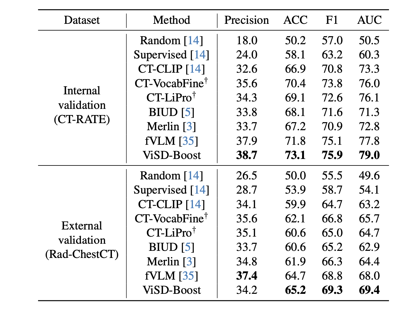
솔직히 이런거 지겹다. AUC 찔끔 올라갔다고 이걸 올리는게맞나? 이런건 워크샵이맞는거같은데.

Ablation Study

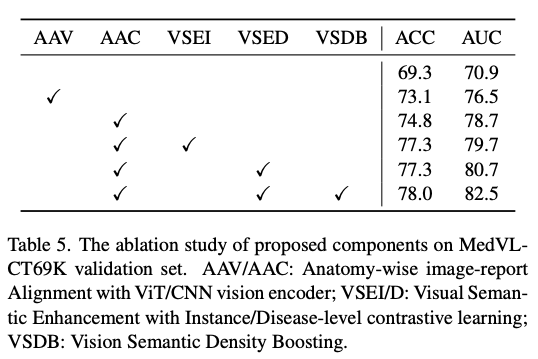
그래도 꼭 필요한 ablation study 는 했다 ~~(안했으면 떨어졌겠지)~~.

fVLM 이랑 달라진게 있다. ViT 대신에 CNN backbone 쓴다 ㅋㅋ
VSE (vision only pretraining) 을 했을 때 AUC 가 2 pt 올라간다. Disease level 이 AUC 가 더 올라간다고 한다.
VSD (VQVAE) 를 쓰면 1.8 pt 더 발전시켰다고 한다.

Qualitative Analysis

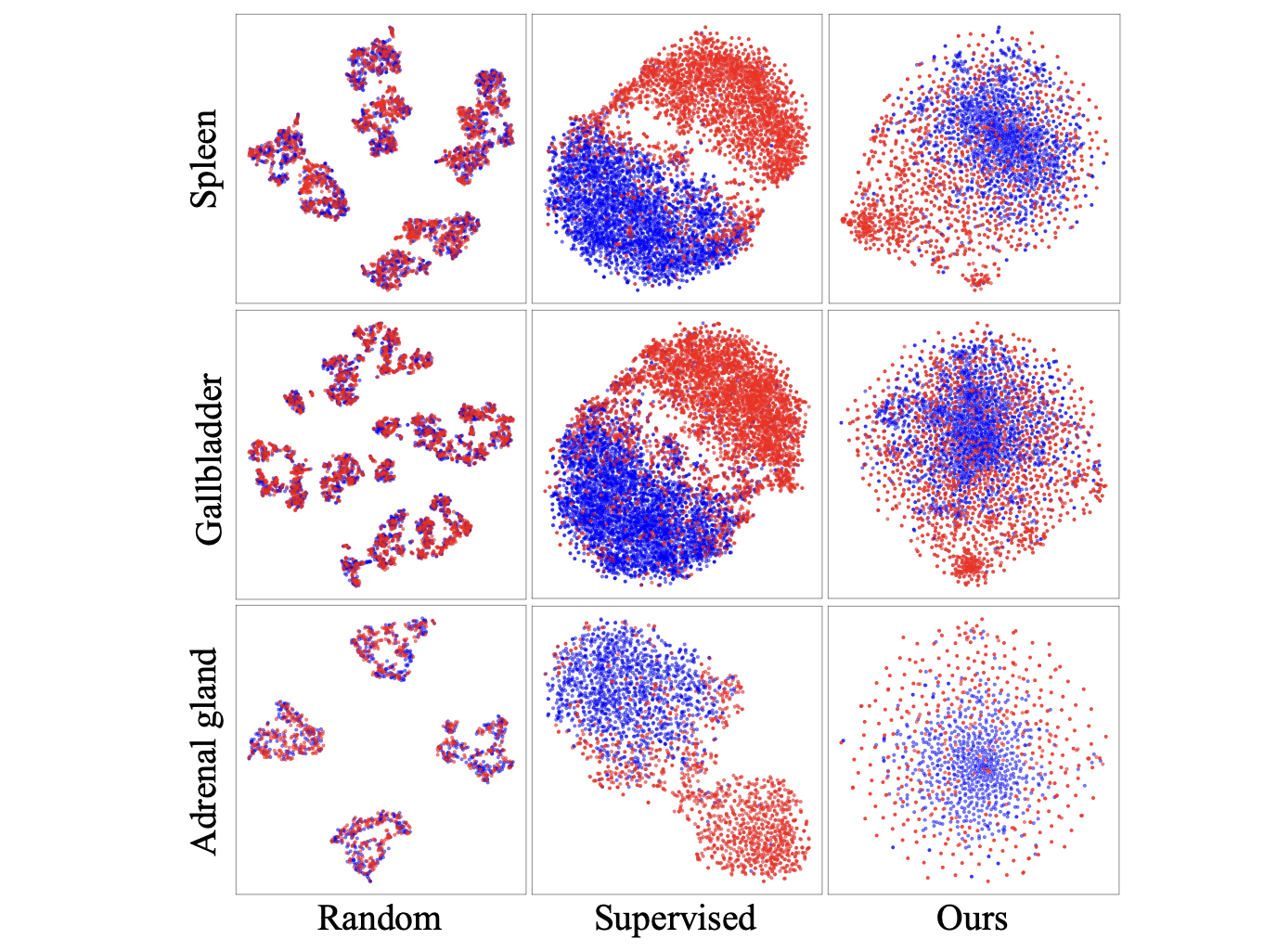
Figure 4 에서는 t-SNE analysis 로 VSE 의 효능을 강조한다. 파란색이 normal, 빨간색이 abnormal 이다. 전반적으로, normal 끼리 뭉쳐있고 disease 는 collapse 돼지 않으면서 퍼져있는 모습이 VSE 의 훈련효과를 납득시킨다.

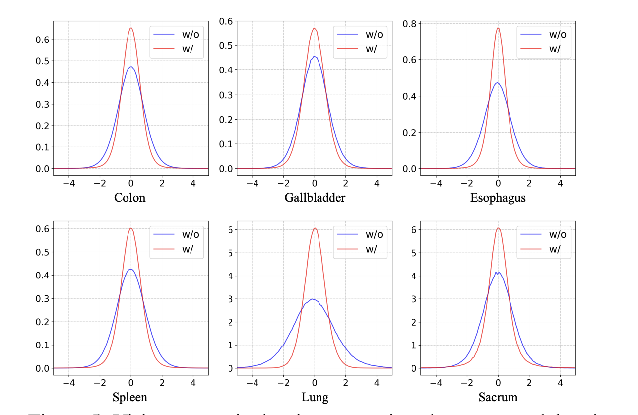
Figure 5 에서는 vision semantic density 로 VSD 의 효능을 강조한다. 근데 의문인게, sparsity 가 증가했다고 해서 richer semantics 가 되는지는 납득이 안된다. 이런 주장을 할거면 localization 을 더 잘한다는 결과를 하나 더 가져오거나, VSD 없이 sparsity 를 encourage 하는 regularization loss 를 넣은 결과랑 비교해야 하지 않을까?