U_Week_2_Day_10

수업 정리 　

강의 목록

[DL Basic] Generative Models 1

• Learning a Generative Model
  • Generation(sampling) : If we sample $x_{new} \sim p(x), x_{new}$ should look like a dog
  • Density estimation(anomaly detection) : $p(x)$ should be high if $x$ looks lik a dog, and low otherwise. also known as, explicit models.
  • Unsupervised representation learning(feature learning) : We should be able to learn what these image have in common, e.g., ears, tail, etc
    >> then, how can we represent $p(x)$?
• Basic Discrete Distributions
  • Bernoulli distribution : (biased) coin flip
    • $D = \{\mathrm{Head, Tails}\}$
    • Specify $P(X = \mathrm{Heads}) = p.$ Then $P(X=\mathrm{Tails}) = 1 - p.$
    • Write : $X \sim \mathrm{Ber}(p)$
  • Categorical distribution : (biased) m-sided dice
    • $D = \{1, ..., m\}$
    • Specify $P(Y=i) = p_{i},$ such that $\sum_{i=1}^m p_{i}=1$
    • Write : $Y \sim \mathrm{Cat}(p_{1}, ..., p_{m})$
• Structure Through Independence
  • What if $X_{1}, ..., X_{n}$ are independent, then $p(x_{1}, ..., x_{n} = p(x_{1})p(x_{2})...p(x_{n})$
  • How many possible states? ${\color{Blue}2^n}$
  • How many parameters to specify $p(x_{1}, ..., x_{n})?$ ${\color{Blue}n}$
  • ${\color{Blue}2^n}$ entries can be described by just ${\color{Blue}n}$ numbers! But this ${\color{Blue}\mathrm{independence}}$ assumption is too strong to model useful distributions.
• Conditional Independence
  • Three important rules
    • Chain rule : $p(x_{1}, ..., x_{n}) = p(x_{1})p(x_{2}|x_{1})p(x_{3}|x_{1},x_{2})...p(x_{n}|x_{1},...,x_{n-1})$
    • Bayes' rule : $p(x|y) = \frac{p(x,y)}{p(y)}=\frac{p(y|x)p(x)}{p(y)}$
    • Conditional independence : If $x \bot y|x,$ then $p(x|y,z)=p(x|z)$
  • If using the chain rule, How many parameters?
    • ${\color{Blue}p(x_{1})}$ : 1 params
    • ${\color{Blue}p(x_{2}|x_{1})}$ : 2 params (one per $p(x_{2}|x_{1} = 0)$ and one per $p(x_{2}|x_{1} = 1)$
    • ${\color{Blue}p(x_{3}|x_{1}, x_{2})}$ : 4 params
    • Hence, $1+2+2^{2}+...+2^{n-1}=2^{n}-1$
    • Now, suppose $X_{i+1} \bot X_{1},...,X_{i-1}|X_{i}$(Markov assumption), then ${\color{Blue}p(x_{1}, ..., x_{n}) = p(x_{1})p(x_{2}|x_{1})p(x_{3}|x_{2})...p(x_{n}|x_{n-1})}$
    • How many parameters? ${\color{Blue}2n-1}$
    • Hence, by leveraging the Markov assumption, we get exponential reduction on the number of parameters.
    • Auto-regressive models leverage this conditional independency.
• Auto-regressive model
  • Suppose we have $28 \times 28$ binary pixels
  • Our goal is to learn $p(x) = p(x_{1}, ..., x_{784})$ over $x \in {0,1}^{784}$
  • How can we parametrize $p(x)$?
    • Let's use the chain rule to factor the joint distribution
    • $p(x_{1:784})=p(x_{1})p(x_{2}|x_{1})p(x_{3}|x_{1:2})...$
    • This is called an autoregressive model
    • Note that we need an order of all random variables.
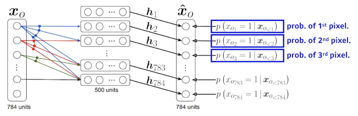
• NADE : Neural Autoregressive Density Estimator
  
  • probability distribution of $i$-th pixel : $p(x_{i}|x_{1:i-1}) = \sigma(a_{i}h_{i} + b{i})$ where $h_{i} = \sigma(W_{<i}x_{1:i-1}+c)$
  • NADE is an explicit model that can compute the density of the given inputs
  • How can we compute the density off the given image?
    • Suppose we have image with 784 binary pixels, $\{x_{1}, x_{2}, ..., x_{784}\}$
    • Then, the joint probability is computed by $\{x_{1}, x_{2}, ..., x_{784}\} = p(x_{1})p(x_{2}|x_{1})...p(x_{784}|x_{1:783})$ where each conditional probability $p(x_{i}|x_{1:i-1})$ is computed independently
  • In case of modeling continuous random variable, a mixture of Gaussian can be used
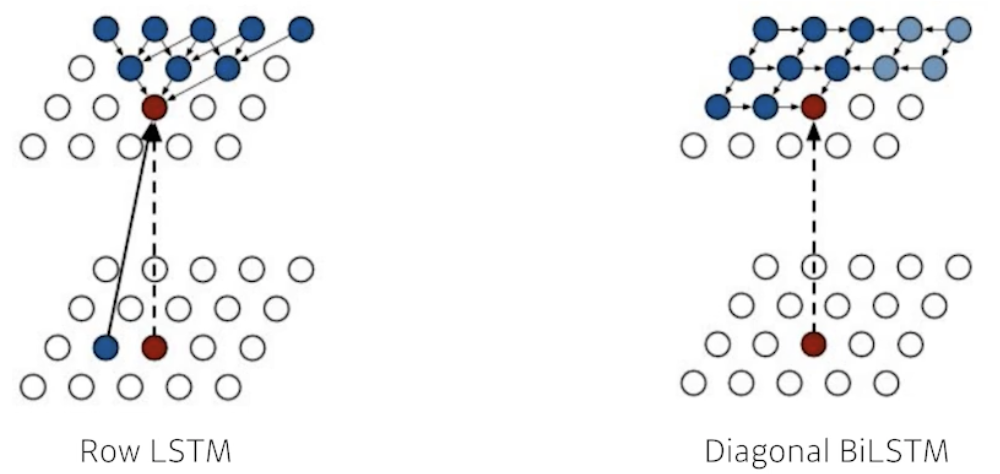
• Pixel RNN
  • We can also use RNNs to define an auto-regressive model
  • For example, for an $n \times n$ RGB image, $p(x) = \prod_{i=1}^{n^2} p(x_{i,R}|x_{<i}p(x_{i,G}|x_{<i},x_{i,R})p(x_{i,B}|x_{<i},x_{i,R},x_{i,G})$
  • There are two model architectures in Pixel RNN based on the ordering of chain:
    • Row LSTM
    • Diagonal BiLSTM
      

[DL Basic] Generative Models 2

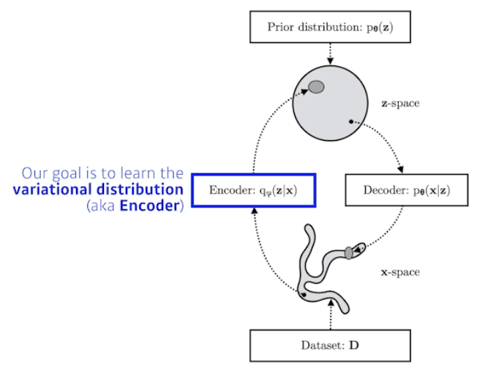
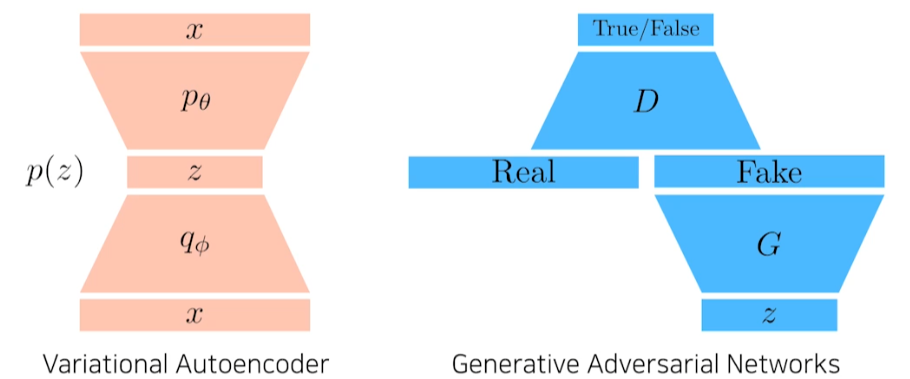
• Variational Auto-encoder
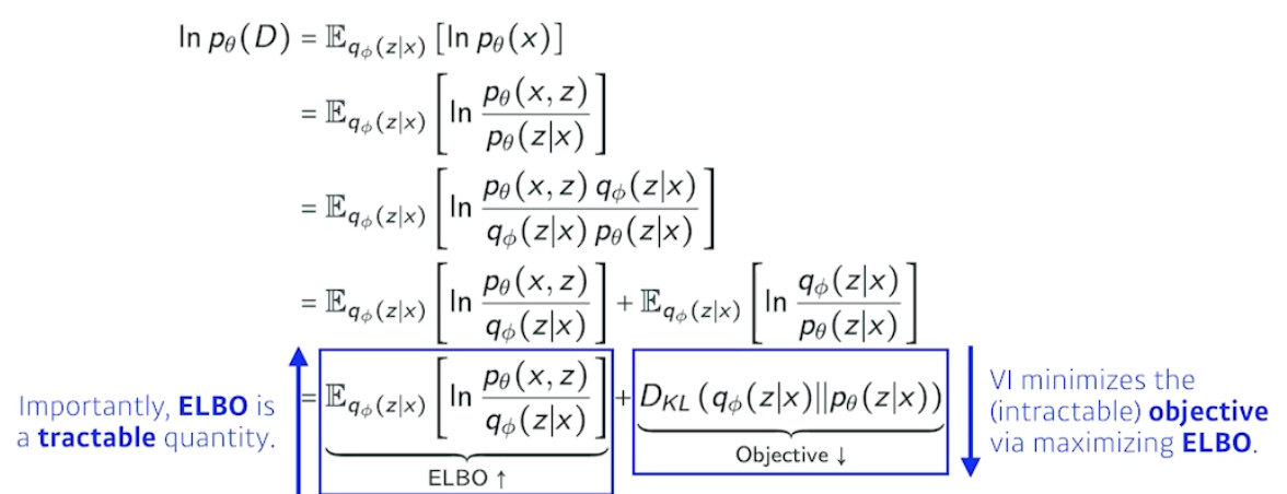
  • Variational inference(VI)
    • The goal of VI is to optimize the variational distribution that best matches the posterior distribution
    • Posterior distribution : $p_{\theta}(z|x)$
    • Variational distribution : $p_{\phi}(z|x)$
    • In particular, we want to find the variational distribution that minimizes the KL divergence between the true posterior
    • 
    • But how?
      
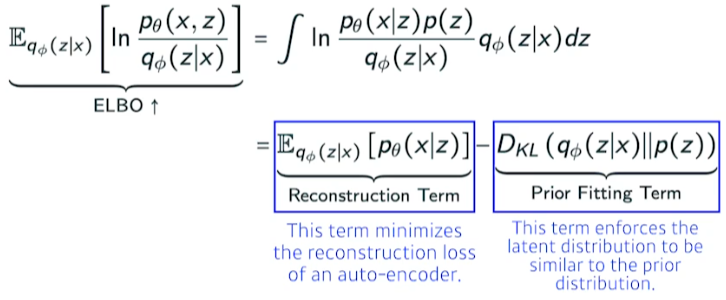
    • ELBO can further be decompsed into
      
  • Key limitation
    • It is an intractable model(hard to evaluate likelihood)
    • The prior fitting term must be differentiable, hence it is hard to use diverse latent prior distributions.
    • In most cases, we us an isotropic Gaussian
      $D_{K L}\left(q_{\phi}(z \mid x) \| \mathcal{N}(0, l)\right)=\frac{1}{2} \sum_{i=1}^{D}\left(\sigma_{z_{i}}^{2}+\mu_{z_{i}}^{2}-\ln \left(\sigma_{z_{i}}^{2}\right)-1\right)$
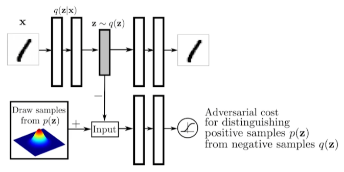
• Adversarial Auto-encoder
  
  • It allows us to use any arbitrary latent distributions that we can sample
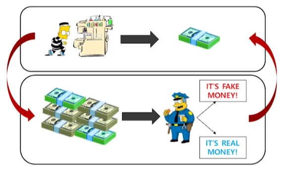
• GAN
  
  • $\min _{G} \max _{D} V(D, G)=\mathbb{E}_{\boldsymbol{x} \sim p_{\text {data }}(\boldsymbol{x})}[\log D(\boldsymbol{x})]+\mathbb{E}_{\boldsymbol{z} \sim p_{\boldsymbol{z}}(\boldsymbol{z})}[\log (1-D(G(\boldsymbol{z})))]$
  • GAN vs VAE
    
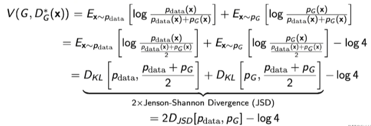
  • GAN Objective
    • A two player minimax game between generator and discriminator
    • For discriminator:
      • $\max _{D} V(G, D)=E_{\mathbf{x} \sim p_{\mathrm{data}}}[\log D(\mathbf{x})]+E_{\mathbf{x} \sim p_{G}}[\log (1-D(\mathbf{x}))]$
      • where the optimal discriminator is $D_{G}^{*}(\mathbf{x})=\frac{p_{\text {data }}(\mathbf{x})}{p_{\text {data }}(\mathbf{x})+p_{G}(\mathbf{x})}$
    • For generator : $\min _{G} V(G, D)=E_{\mathbf{x} \sim p_{\text {data }}}[\log D(\mathbf{x})]+E_{\mathbf{x} \sim p_{G}}[\log (1-D(\mathbf{x}))]$
    • Plugging in the optimal discriminator, we get
      
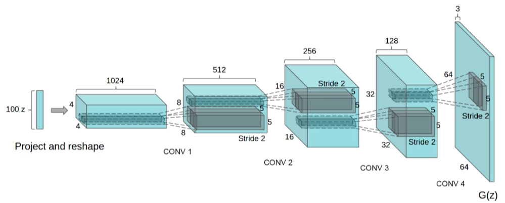
• DCGAN
  
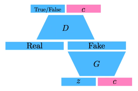
• Info-GAN
  
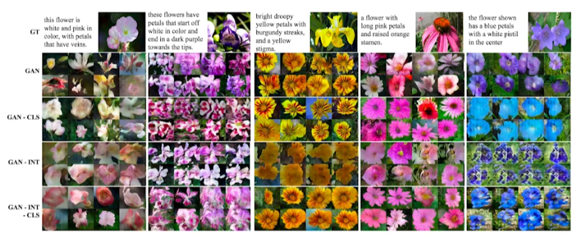
• Text2Image
  
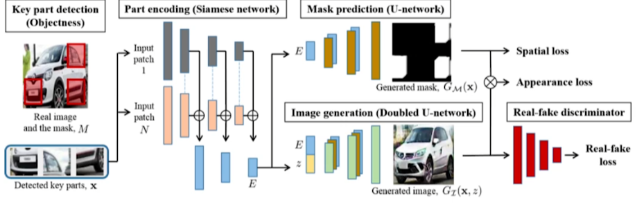
• Puzzle-GAN
  
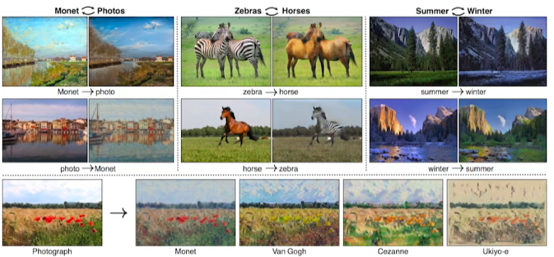
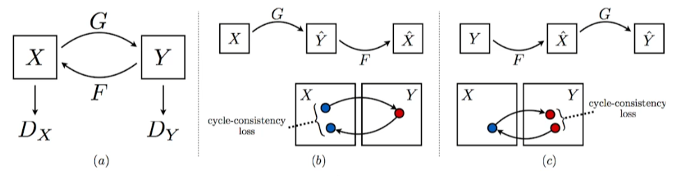
• CycleGAN
  
  • Cycle-consistency loss
    
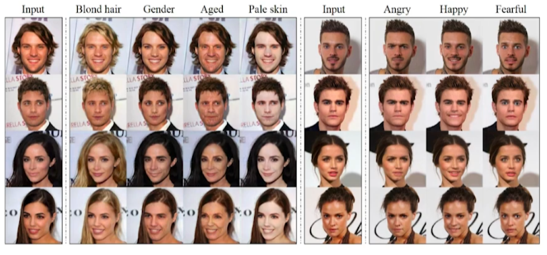
• Star-GAN
  
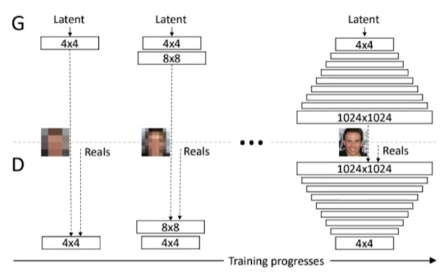
• Progressive-GAN
  

피어세션 정리

• 스페셜 피어세션
• 팀 회고록 작성

느낀점

기존에 공부했던 NLP외에 CNN 발전 모델과 GAN 등을 공부할 수 있었던 일주일이었습니다.

벌써 2주가 지났습니다. 목표로하던 대회, 공모전 참가는 아직 실행에 옮기지 못했습니다... 하루 빨리 대회 찾아서 참가라도 해보는 것에 의의를 두어야 할 것 같습니다.