20220106(목)
머신러닝 절차
- 데이터 가져오기
- 모델 학습하기 위한 데이터 나누기
- 모델 학습하기
- 모델 평가하기
- 정리
- 그 외에
1. 데이터 가져오기
사용하는 패키지
pip install scikit-learn # 데이터
pip install matplotlib # 시각화-> 좌측에 User Guide의 7. Dataset loading utilites를 참고하자
데이터 살펴보기
- 데이터 가져오기
from sklearn.datasets import load_iris

iris = load_iris()

print(dir(iris))
# dir() 함수로 해당 객체의 변수와 메소드 확인
>>> ['DESCR', 'data', 'data_module', 'feature_names', 'filename', 'frame', 'target', 'target_names']

iris.keys()
>>> dict_keys(['data', 'target', 'frame', 'target_names', 'DESCR', 'feature_names', 'filename', 'data_module'])- 데이터 형태
iris_data = iris.data
print(iris_data.shape)
# shape써서 data의 행렬을 보여줌
# 150개의 데이터가 4개의 정보를 갖고 있음
>>> (150, 4)- 데이터의 인덱스 값 확인
iris_data[0]
# data의 0번째 인덱스 값
>>> array([5.1, 3.5, 1.4, 0.2])- 데이터 라벨링
iris_label = iris.target
iris_label
# 호출할 때 target으로 호출함
>>> array([0, 0, 0, 0, 0, 0, 0, 0, 0, 0, 0, 0, 0, 0, 0, 0, 0, 0, 0, 0, 0, 0,
       0, 0, 0, 0, 0, 0, 0, 0, 0, 0, 0, 0, 0, 0, 0, 0, 0, 0, 0, 0, 0, 0,
       0, 0, 0, 0, 0, 0, 1, 1, 1, 1, 1, 1, 1, 1, 1, 1, 1, 1, 1, 1, 1, 1,
       1, 1, 1, 1, 1, 1, 1, 1, 1, 1, 1, 1, 1, 1, 1, 1, 1, 1, 1, 1, 1, 1,
       1, 1, 1, 1, 1, 1, 1, 1, 1, 1, 1, 1, 2, 2, 2, 2, 2, 2, 2, 2, 2, 2,
       2, 2, 2, 2, 2, 2, 2, 2, 2, 2, 2, 2, 2, 2, 2, 2, 2, 2, 2, 2, 2, 2,
2, 2, 2, 2, 2, 2, 2, 2, 2, 2, 2, 2, 2, 2, 2, 2, 2, 2])- 데이터 라벨링의 이름
iris.target_names
# target_names를 통해 데이터 라벨링 이름을 알 수 있다
>>> array(['setosa', 'versicolor', 'virginica'], dtype='<U10') - 데이터셋 설명
print(iris.DESCR)
# DESCR 함수를 통해 데이터셋의 설명을 볼 수 있다
>>> .. _iris_dataset:

Iris plants dataset
--------------------

**Data Set Characteristics:**

    :Number of Instances: 150 (50 in each of three classes)
    :Number of Attributes: 4 numeric, predictive attributes and the class
    :Attribute Information:
        - sepal length in cm
        - sepal width in cm
        - petal length in cm
        - petal width in cm
        - class:
                - Iris-Setosa
                - Iris-Versicolour
                - Iris-Virginica
...- 데이터 feature 설명
iris.feature_names
>>>
['sepal length (cm)',
 'sepal width (cm)',
 'petal length (cm)',
 'petal width (cm)']
2. 모델 학습하기 위한 데이터 나누기
라이브러리 불러오기
import pandas as pd배열 데이터를 다루는데 pandas를 사용할 예정이다.
원래 이 과정에서 전처리도 이루어지는데 이번에 불러오는 데이터는 정리가 다 되어있어서 따로 하지 않는다.
- 배열 만들기
iris_df = pd.DataFrame(data=iris_data, columns=iris.feature_names) # 배열 만들기
iris_df["label"] = iris.target # 라벨 붙이기
iris_df
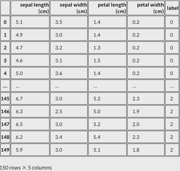
pandas의 DataFrame을 이용해 2차원 배열을 만들었다.
row=iris_data, columns=iris.feature_names를 사용했다.
가장 우측에 label을 통해 정답지도 같이 추가했다.
feature, label(target)을 이해하고 가자
- 데이터 분리하기
현재 총 150개의 데이터셋을 갖고 있다.
머신러닝 모델은 학습용 데이터와 테스트용 데이터는 겹치면 안되기 때문에 training dataset과 test dataset으로 나눠야 한다.
from sklearn.model_selection import train_test_split

X_train, X_test, y_train, y_test = train_test_split(iris_data,
                                                    iris_label,
                                                    test_size=0.2,
                                                    random_state=7)

print('X_train 개수: ', len(X_train),', X_test 개수: ', len(X_test))

>>> X_train 개수:  120 , X_test 개수:  30
train_test_split 기능으로 손 쉽게 나눌 수 있다.
*_train은 트레이닝용으로 후에 모델을 만들 때 사용된다. x_train은 row값, y_train은 label값을 갖고 있다.
test_size=0.2로 total 150EA의 20%인 30개의 데이터를 *_test으로 보냈다.
여기서 random_state는 y_train이 갖고있는 해시값이라고 보면 편하다.
랜덤으로 테스트용 데이터를 추출하지만 해시값을 같게 해서 재현할 수 있다.(해당 인자는 없어도 무관하다.)
- 데이터셋 확인하기
X_train.shape, y_train.shape
>>> ((120, 4), (120,))

X_test.shape, y_test.shape
>>> ((30, 4), (30,))

y_train, y_test
>>> (array([2, 1, 0, 2, 1, 0, 0, 0, 0, 2, 2, 1, 2, 2, 1, 0, 1, 1, 2, 0, 0, 0,
        2, 0, 2, 1, 1, 1, 0, 0, 0, 1, 2, 1, 1, 0, 2, 0, 0, 2, 2, 0, 2, 0,
        1, 2, 1, 0, 1, 0, 2, 2, 1, 0, 0, 1, 2, 0, 2, 2, 1, 0, 1, 0, 2, 2,
        0, 0, 2, 1, 2, 2, 1, 0, 0, 2, 0, 0, 1, 2, 2, 1, 1, 0, 2, 0, 0, 1,
        1, 2, 0, 1, 1, 2, 2, 1, 2, 0, 1, 1, 0, 0, 0, 1, 1, 0, 2, 2, 1, 2,
        0, 2, 1, 1, 0, 2, 1, 2, 1, 0]),
 array([2, 1, 0, 1, 2, 0, 1, 1, 0, 1, 1, 1, 0, 2, 0, 1, 2, 2, 0, 0, 1, 2,
        1, 2, 2, 2, 1, 1, 2, 2]))
y_train과 y_test는 train_test_split 덕분에 label값이 무작위로 섞여있다.
이제 모델을 학습시키면 된다!
3. 모델 학습하기
Decision Tree(의사결정나무) 학습법
관련 내용을 더 확인하고 싶으면 아래 사이트를 참고하자
from sklearn.tree import DecisionTreeClassifier

decision_tree = DecisionTreeClassifier(random_state=32)
전에 만들어둔X_train = row값과 y_train = row 라벨링 한 데이터로 쉽게 학습할 수 있다.
decision_tree.fit(X_train, y_train)이 때 메서드 이름이 fit인데 이는 training dataset에서 패턴을 파악하고 이에 맞게 예측할 수 있도록 모델을 fitting한다는 것을 의미한다.
4. 모델 평가하기
y_pred = decision_tree.predict(X_test)
y_pred
>>> array([2, 1, 0, 1, 2, 0, 1, 1, 0, 1, 2, 1, 0, 2, 0, 2, 2, 2, 0, 0, 1, 2,
       1, 1, 2, 2, 1, 1, 2, 2])
학습이 완료된 decision_tree 모델에 row값만 있었던 X_test를 넣고 predict하면 예측값 y_pred를 얻게된다.
y_test
>>> array([2, 1, 0, 1, 2, 0, 1, 1, 0, 1, 1, 1, 0, 2, 0, 1, 2, 2, 0, 0, 1, 2,
1, 2, 2, 2, 1, 1, 2, 2])- 정확도(Accuracy) 확인하는 방법
from sklearn.metrics import accuracy_score

accuracy = accuracy_score(y_test, y_pred)
accuracy

>>> 0.9
0.9는 90%라는 뜻이다. 이를 다시 생각하면 30개의 테스트 데이터 중 27개만 맞았고 3개만 틀렸다는 의미다.
(예측이 정답인 데이터 수 / 예측한 전체 데이터 수)5. 정리
# (1) 모듈 import
from sklearn.datasets import load_iris
from sklearn.model_selection import train_test_split
from sklearn.tree import DecisionTreeClassifier
from sklearn.metrics import classification_report

# (2) 데이터 준비
iris = load_iris()
iris_data = iris.data
iris_label = iris.target

# (3) 학습, 시험용 데이터 분리
X_train, X_test, y_train, y_test = train_test_split(iris_data,
                                                    iris_label,
                                                    test_size=0.2,
                                                    random_state=7)

# (4) 모델 학습 및 예측
decision_tree = DecisionTreeClassifier(random_state=32)
decision_tree.fit(X_train, y_train)
y_pred = decision_tree.predict(X_test)

print(classification_report(y_test, y_pred))

>>>
              precision    recall  f1-score   support

           0       1.00      1.00      1.00         7
           1       0.91      0.83      0.87        12
           2       0.83      0.91      0.87        11

    accuracy                           0.90        30
   macro avg       0.91      0.91      0.91        30
weighted avg       0.90      0.90      0.90        30
1 ~ 3번은 흐름이 크게 바뀌지 않고 모델을 추가하거나 바꾸고 싶으면 4번 부분만 바꿔주면 된다!
+ 추가 모델
- Random Forest
의사결정 나무를 여러 개 모아놓은 형태로 단점을 앙상블(Ensemble) 기법으로 극복한 모델이다.
관련 추가 내용은 Random Forest 개념 정리를 참고하자
from sklearn.ensemble import RandomForestClassifier

X_train, X_test, y_train, y_test = train_test_split(iris_data,
                                                    iris_label,
                                                    test_size=0.2,
                                                    random_state=21)

random_forest = RandomForestClassifier(random_state=32)
random_forest.fit(X_train, y_train)
y_pred = random_forest.predict(X_test)

print(classification_report(y_test, y_pred))

>>>
              precision    recall  f1-score   support

           0       1.00      1.00      1.00        11
           1       1.00      0.83      0.91        12
           2       0.78      1.00      0.88         7

    accuracy                           0.93        30
   macro avg       0.93      0.94      0.93        30
weighted avg       0.95      0.93      0.93        30
이 또한 sklearn.ensemble 패키지를 이용하면 손 쉽게 구현할 수 있다.
- Support Vector Machine(SVM)
Hyperplane(초평면)을 이용해서 분류하는 대표적인 선형 분류 알고리즘

sklearn 패키지를 이용한 SVM 구현 방법
from sklearn import svm
svm_model = svm.SVC()

svm_model.fit(X_train, y_train)
y_pred = svm_model.predict(X_test)

print(classification_report(y_test, y_pred))

>>>
실행 완료
              precision    recall  f1-score   support

           0       1.00      1.00      1.00        11
           1       0.91      0.83      0.87        12
           2       0.75      0.86      0.80         7

    accuracy                           0.90        30
   macro avg       0.89      0.90      0.89        30
weighted avg 0.91 0.90 0.90 30- Stochastic Gradient Descent Classifier(SGDClassifier)
확률적 경사하강법
from sklearn.linear_model import SGDClassifier
sgd_model = SGDClassifier()

sgd_model.fit(X_train, y_train)
y_pred = sgd_model.predict(X_test)

print(classification_report(y_test, y_pred))- Logistic Regression
선형 분류 알고리즘으로 로지스틱 회귀 또는 소프트맥스 회귀(Softmax Regression)
from sklearn.linear_model import LogisticRegression
logistic_model = LogisticRegression()

from sklearn.ensemble import RandomForestClassifier

from sklearn.ensemble import RandomForestClassifier

X_train, X_test, y_train, y_test = train_test_split(iris_data,
                                                    iris_label,
                                                    test_size=0.2,
                                                    random_state=15)

decision_tree = RandomForestClassifier(random_state=2)
decision_tree.fit(X_train, y_train)
y_pred = decision_tree.predict(X_test)

print(accuracy_score(y_test, y_pred))
위의 두 알고리즘도 sklearn을 이용해서 손쉽게 모델을 학습하고 구현해낼 수 있었다.
6. 그 외에
- 오차 행렬(confusion matrix)을 표현하는 방법
참고 사이트
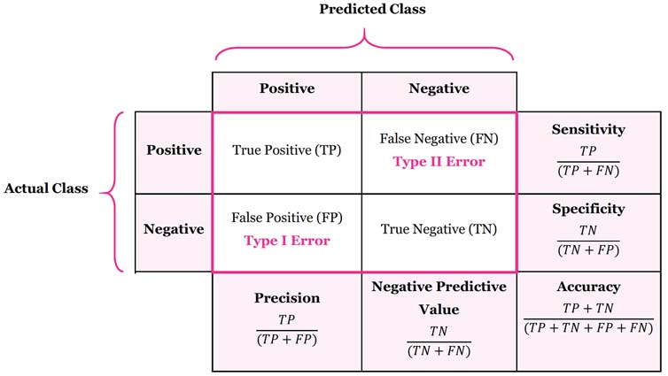
좌측에 Actual Class는 실제 클래스를 나타내고 상단에 Predicted Class는 예측된 클래스를 나타낸다.
예측 결과는 TP, FP, TN, FN 네가지로 나뉜다.
Positive가 양성, Negative가 음성이라고 예를 들었을 때 예측 결과는 다음과 같다.
- TP(True Positive) : 환자에게 양성
- FN(False Negative) : 환자에게 음성
- FP(False Positive) : 건강한 사람에게 양성
- TN(True Negative) : 건강한 사람에게 음성
Precision이 크려면 음성인데 양성으로 판단하는 경우가 적어야한다.
이는 스팸 메일함에 대조해볼 수 있다.
Sensitivity가 크려면 양성인데 음성으로 판단하는 경우가 적어야한다.
환자에게 대조해볼 수 있다.
이렇게 모델의 성능은 정확도로만 평가하면 안되는 상황이 있을 수 있다.
분류 성능 평가
사이킷런 패키지는 metrics 서브패키지에서 다음처럼 다양한 분류용 성능평가 명령을 제공한다.
confusion_matrix(y_true, y_pred)accuracy_score(y_true, y_pred)precision_score(y_true, y_pred)recall_score(y_true, y_pred)fbeta_score(y_true, y_pred, beta)f1_score(y_true, y_pred)classfication_report(y_true, y_pred)roc_curveauc
