시계열분석 2차시 모델링
목차
1. TG vs not TG
2. 전처리 과정
3. catboost 모델 설명
4. 모델링 과정
1. TG vs not TG
https://dacon.io/competitions/official/236176/codeshare/9381
모델링 과정에서 대회 수상팀 "B부터 N까지"의 코드를 참고하였습니다.
전처리 과정에서 감귤과 감귤이 아닌 것을 따로 모델링하였는데, 두드러지는 특성 차이로 다음 두 가지가 있었습니다.
1) 가격의 범위가 넓다
2) 가격의 0값이 아닌 데이터 비율이 높다
두 번째 특성의 경우 조원들끼리 EDA를 진행해보았을 때 생각하지 못한 부분이었습니다!
첫 번째 특성의 경우 이를 조정하기 위하여 전처리 과정에서 가격에 root를 씌웠습니다.
2. 전처리 과정
2-1. 극단적 이상치 처리
# 극 이상치 제거
tg_idx = train_pre[(train_pre["item"]=="TG") & (train_pre["price"]>20000)].index
rd_idx = train_pre[(train_pre["item"]=="RD") & (train_pre["price"]>5000)].index
bc_idx = train_pre[(train_pre["item"]=="BC") & (train_pre["price"]>8000)].index
cb_idx = train_pre[(train_pre["item"]=="CB") & (train_pre["price"]>2300)].index

train_pre.loc[tg_idx,"price"] = train_pre[(train_pre["item"]=="TG") & (train_pre["price"]!=0)]["price"].mean()
train_pre.loc[rd_idx,"price"] = train_pre[(train_pre["item"]=="RD") & (train_pre["price"]!=0)]["price"].mean()
train_pre.loc[bc_idx,"price"] = train_pre[(train_pre["item"]=="BC") & (train_pre["price"]!=0)]["price"].mean()
train_pre.loc[cb_idx,"price"] = train_pre[(train_pre["item"]=="CB") & (train_pre["price"]!=0)]["price"].mean()
각 품목(item)에 대해 극단적인 가격(price) 값을 가진 행의 인덱스를 추출한 후, 품목별 평균값으로 대체하였습니다.
2-2. TG 전처리
# train 및 test 시간 순서로 정렬하기
train_tg = train_pre[train_pre["item"] == "TG"].sort_values(by = ["timestamp"]).reset_index(drop= True)
test_tg = test_pre[test_pre["item"] == "TG"].sort_values(by = ["timestamp"]).reset_index(drop= True)

Xy = pd.get_dummies(train_tg, columns = [ "item","corporation","location"]).drop(columns = ["supply"])
answer_tg1 = pd.get_dummies(test_tg, columns = [ "item","corporation","location"]).drop(columns = ["timestamp","supply","price"])
print(f"train의 컬럼 : {Xy.columns}")
print(f"test의 컬럼 : {answer_tg1.columns}")

##루트->편차 줄임
Xy["price"] = np.sqrt(Xy["price"])
감귤의 경우 np.sqrt를 해주어 가격의 편차를 줄였습니다.
3. catboost 모델 설명
모델링 과정에서 사용한 catboost 모델에 대해서 간략히 설명하겠습니다.
catboost는 yandex에서 개발한 gradient boosting 알고리즘입니다.
gradient boosting은 boosting의 일종이고, boosting은 앙상블 기법 중 하나입니다.
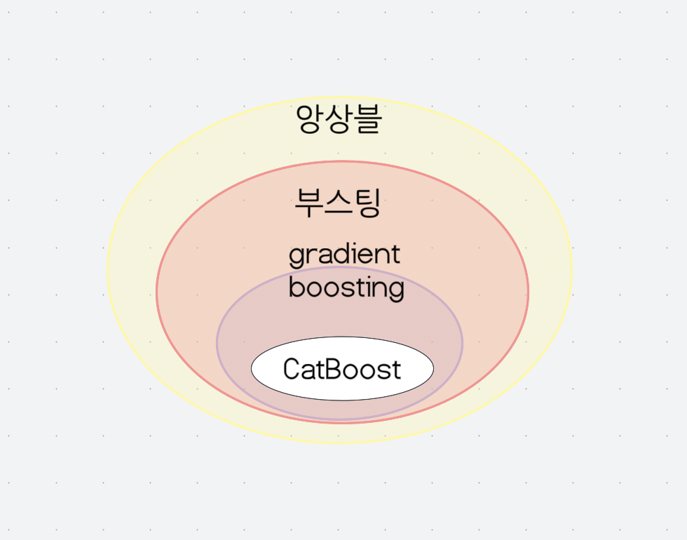
앙상블 idea
개별적으로 어느 정도 좋은 성능을 가지면서, 앙상블 내에서 각각 다양한 형태를 가지는 모델들을 결합하면 서로 다른 사고방식 체계를 가지고 있어 상호 보완이 가능함
부스팅
편향 감소에 의한 오류 감소
현재 모델이 잘 해결하지 못하는 어려운 케이스에 집중하여 앞선 모델 평가 후 다음 모형을 학습하는 방식
gradient boosting
gradient descent + boosting
회귀모형의 잔차를 다음 단계에서 학습하는 모델을 구축
catboost 특징
1) 범주형 변수 처리 가능
2) ordered boosting 방식 사용하여 데이터 순서에 따른 과적합 방지
3) 결측치, 카테고리, 파라미터 튜닝을 자동으로 처리함
4. 모델링 과정
not TG
# CatBoost 모델 정의
cat = CatBoostRegressor(
    random_state=2024,
    n_estimators=1000,
    learning_rate=0.01,
    depth=10,
    l2_leaf_reg=3,
    metric_period=1000
)

# 학습 데이터 및 타겟 분리 (timestamp, ID, price 컬럼 제외)
X = Xy.drop(columns=["timestamp", "ID", "price"])
y = Xy["price"]

# 모델 학습
cat.fit(X, y)

# 예측 데이터에서 ID 컬럼 제외
X_test = answer_notg.drop(columns=["ID"])

# 예측
pred = cat.predict(X_test)

# 예측 값이 0보다 작은 경우 0으로 수정
pred = np.maximum(pred, 0)

# 예측 값을 answer 컬럼에 저장
answer_notg["answer"] = pred

# 결과 출력 (ID와 예측 값)
result = answer_notg[["ID", "answer"]]
print(result)
TG
from catboost import CatBoostRegressor
import numpy as np

# CatBoost 모델 정의
cat = CatBoostRegressor(
    random_state=2024,
    n_estimators=1000,
    learning_rate=0.01,
    depth=10,
    l2_leaf_reg=3,
    metric_period=1000
)

# 학습 데이터 및 타겟 분리 (timestamp, ID, price 컬럼 제외)
X = Xy.drop(columns=["timestamp", "ID", "price"])
y = Xy["price"]

# 모델 학습
cat.fit(X, y)

# 예측 데이터에서 ID 컬럼 제외
X_test = answer_tg1.drop(columns=["ID"])

# 예측
pred = cat.predict(X_test)

# 예측 값이 0보다 작은 경우 0으로 수정
pred = np.maximum(pred, 0)

# 예측 값을 제곱하여 저장
########TG만 price에 폭이 커서 처음에 루트 씌웠기 때문에 나중에 다시 제곱
answer_tg1["answer"] = np.power(pred, 2)

# 결과 출력 (ID와 예측 값)
result = answer_tg1[["ID", "answer"]]
print(result)