- 자료출처 : PyTorch로 시작하는 딥 러닝 입문
인공신경망
- 인공신경망은 머신러닝 방법 중 하나이다. 하지만 최근 인공신경망을 복잡하게 쌓아올린 딥러닝이 다른 머신러닝을 뛰어넘는 성능을 보여주며 자주 활용되고 있다.
- 딥러닝도 머신러닝의 일부이므로 머신러닝의 특징을 먼저 정리한다.
1. 머신러닝의 특징
1) 머신러닝 모델의 평가
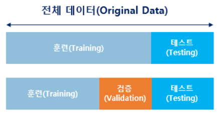
- 실제 모델을 평가하기 위해선 데이터를 훈련용, 검증용, 테스트용으로 세 가지로 분리한다.
- 검증용 데이터는 모델의 성능을 평가하기 보단 모델의 성능을 조정하기 위한 용도다.
(더 정확히는 과적합이 되고 있는지 판단하거나 하이퍼파라미터의 조정을 위한 용도) - 하이퍼파라미터는 값에 따라 모델의 성능에 영향을 주는 매개변수들을 의미
- 반면 가중치와 편향과 같이 학습을 통해 바뀌는 변수는 매개변수라고 부른다.
하이퍼파라미터는 사용자가 직접 정해줄 수 있는 변수고, 매개변수는 모델이 학습하는 과정에서 얻어지는 값이라는 점이 가장 큰 차이다. 훈련용 데이터로 훈련을 모두 시킨 모델은 검증용 데이터를 사용하여 정확도를 검증하며 하이퍼파라미터를 튜닝한다.
2) 정밀도와 재현율
- 전체 문제 중 맞춘 문제 수만을 가지고 산출하는 정확도는 세부 내용을 보여주지 못함
- 그래서 자주 쓰이는게 정밀도와 재현율인데, 이를 위해 사용하는 것이 혼동행렬이다.

- 1행은 예측이 양성(Positive)인지 음성(Nagative)인지
- 1열은 예측결과가 정답(True)인지 오답(False) 인지
- TP는 양성으로 예측했는데 정답, FP는 양성으로 에측했는데 오답인 경우
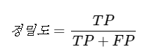
- 정밀도는 양성이라고 대답한 케이스 중 맞춘 비율
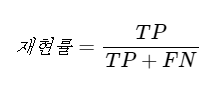
- 재현율은 전체 양성 데이터 중 얼마나 양성으로 예측했는지 나타냄
2. 퍼셉트론 (Perceptron)
- 퍼셉트론은 초기 형태의 인공신경망으로 실제 뇌를 구성하는 신경세포 뉴런의 동작과 유사하다.
- 뉴런은 가지돌기에서 신호를 받아들이고, 이 신호가 일정치 이상의 크기를 가지면 축삭돌기를 통해서 신호를 전달한다.
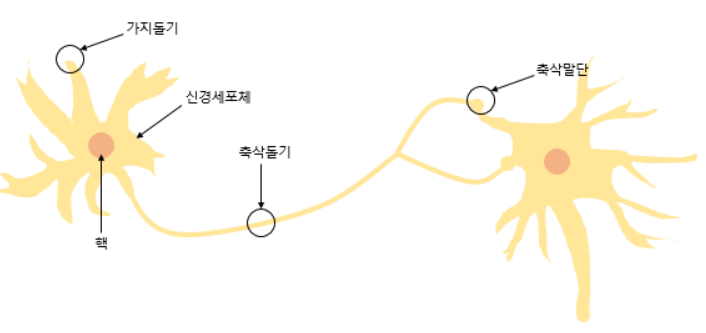
- 퍼셉트론의 그림을 보면 다수의 입력으로부터 하나의 결과를 내보낸다.
- 신경세포 뉴런의 입력 신호와 출력신호가 퍼셉트론에서 각각 입력값과 출력값에 해당된다.
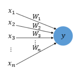
- x는 입력값을 의미하며, W는 가중치(클수록 입력값이 중요) y는 출력값
- 그림 안의 원은 인공뉴런에 해당 / 촉삭돌기의 역할은 퍼셉트론에서의 가중치가 대신함
- 입력값 x는 가중치 W이 함께 종착지인 인공뉴런에 전달
- 입력값과 가중치의 곱의 전체 합이 임게치를 넘으면 인공뉴런은 1을 출력하고, 그렇지 않으면 0을 출력
- 이런 함수를 계단함수라고 한다. (아래는 예시)
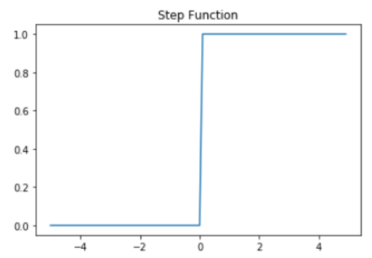
- 뉴런에서 출력값을 변경시키는 함수를 활성화 함수라고 한다.
- 초기 인공신경망 모델인 퍼셉트론은 활성화 함수로 계단함수를 사용하였지만,
- 이후 발전된 신경망들은 계단함수 외에도 다양한 활성화 함수를 사용하기 시작
(시그모이드 함수나 소프트맥스 함수도 활성화 함수) - 로지스틱 회귀를 수행하는 인공뉴런과 퍼셉트론의 차이는 오직 활성화 함수의 차이
3. 단층퍼셉트론 구현 (XOR 문제)
- 퍼셉트론은 단층과 다층으로 나뉘는데, 단층은 위에서 본 것처럼 입력층과 출력층으로만 이루어진다.
(직선 하나로 두 영역을 나눌 수 있는 문제에 대해서만 구현이 가능) - 다층 퍼셉트론(MLP)은 은닉층이 존재해 단층퍼셉트론보다 더 복잡한 문제의 해결이 가능하다.
import torch
import torch.nn as nn
device = 'cuda' if torch.cuda.is_available() else 'cpu'
# GPU 연산이 가능하면 GPU 연산 수행
torch.manual_seed(777)
if device == 'cuda':
torch.cuda.manual_seed_all(777)# XOR 문제에 해당하는 입력과 출력 정의
X = torch.FloatTensor([[0, 0], [0, 1], [1, 0], [1, 1]]).to(device)
Y = torch.FloatTensor([[0], [1], [1], [0]]).to(device)# 1개의 뉴런을 가지는 단층 퍼셉트론
linear = nn.Linear(2, 1, bias=True)
sigmoid = nn.Sigmoid()
model = nn.Sequential(linear, sigmoid).to(device)# 비용 함수와 옵티마이저 정의
criterion = torch.nn.BCELoss().to(device)
optimizer = torch.optim.SGD(model.parameters(), lr=1)#10,001번의 에포크 수행. 0번 에포크부터 10,000번 에포크까지.
for step in range(10001):
optimizer.zero_grad()
hypothesis = model(X)
# 비용 함수
cost = criterion(hypothesis, Y)
cost.backward()
optimizer.step()
if step % 1000 == 0: # 1000번째 에포크마다 비용 출력
print(step, cost.item()) # 비용이 줄어드는 과정0 0.6931471824645996
1000 0.6931471824645996
2000 0.6931471824645996
3000 0.6931471824645996
4000 0.6931471824645996
5000 0.6931471824645996
6000 0.6931471824645996
7000 0.6931471824645996
8000 0.6931471824645996
9000 0.6931471824645996
10000 0.6931471824645996# 학습된 단층 퍼셉트론으로 예측값 확인
with torch.no_grad():
hypothesis = model(X)
predicted = (hypothesis > 0.5).float()
accuracy = (predicted == Y).float().mean()
print('모델의 출력값(Hypothesis): ', hypothesis.detach().cpu().numpy())
print('모델의 예측값(Predicted): ', predicted.detach().cpu().numpy())
print('실제값(Y): ', Y.cpu().numpy())
print('정확도(Accuracy): ', accuracy.item())모델의 출력값(Hypothesis): [[0.5]
[0.5]
[0.5]
[0.5]]
모델의 예측값(Predicted): [[0.]
[0.]
[0.]
[0.]]
실제값(Y): [[0.]
[1.]
[1.]
[0.]]
정확도(Accuracy): 0.5- 실제값은 0,1,1,0 임에도 잘못된 결과를 출력한다. 단층 퍼셉트론으로는 XOR 문제를 풀지 못함
# MNIST dataset
mnist_train = dsets.MNIST(root='MNIST_data/',
                          train=True,
                          transform=transforms.ToTensor(),
                          download=True)

mnist_test = dsets.MNIST(root='MNIST_data/',
                         train=False,
                         transform=transforms.ToTensor(),
                         download=True)
# dataset loader
data_loader = DataLoader(dataset=mnist_train,
batch_size=batch_size, # 배치 크기는 100
shuffle=True,
drop_last=True)- DataLoader(dataset 로드할 대상, 배치사이즈, 셔플여부, 마지막 배치를 버릴지 여부)
- drop_last를 하는 이유는 마지막 배치가 과대평가되는 현상을 막기 위해서다.
(1,000개의 데이터를 128개로 나눴을 때 마지막 배치는 104개가 과대평가 될 확률이 높다)
# 모델 설계 : to()는 연산을 어디서 수행할 지 정한다.
# bias는 기본값이 True이므로 표시할 필요는 없지만 명시적으로 표시해줌

# MNIST data image of shape 28 * 28 = 784
linear = nn.Linear(784, 10, bias=True).to(device)
# 비용 함수와 옵티마이저 정의
criterion = nn.CrossEntropyLoss().to(device) # 내부적으로 소프트맥스 함수를 포함하고 있음.
optimizer = torch.optim.SGD(linear.parameters(), lr=0.1)for epoch in range(training_epochs): # 앞서 training_epochs의 값은 15로 지정함.
avg_cost = 0
total_batch = len(data_loader)
for X, Y in data_loader:
# 배치 크기가 100이므로 아래의 연산에서 X는 (100, 784)의 텐서가 된다.
X = X.view(-1, 28 * 28).to(device)
# 레이블은 원-핫 인코딩이 된 상태가 아니라 0 ~ 9의 정수.
Y = Y.to(device)
optimizer.zero_grad()
hypothesis = linear(X)
cost = criterion(hypothesis, Y)
cost.backward()
optimizer.step()
avg_cost += cost / total_batch
print('Epoch:', '%04d' % (epoch + 1), 'cost =', '{:.9f}'.format(avg_cost))
print('Learning finished')Epoch: 0001 cost = 0.535899699
Epoch: 0002 cost = 0.359200478
Epoch: 0003 cost = 0.331210256
Epoch: 0004 cost = 0.316642910
Epoch: 0005 cost = 0.306912184
Epoch: 0006 cost = 0.300341636
Epoch: 0007 cost = 0.295203745
Epoch: 0008 cost = 0.290808439
Epoch: 0009 cost = 0.287419200
Epoch: 0010 cost = 0.284378737
Epoch: 0011 cost = 0.281997472
Epoch: 0012 cost = 0.279780537
Epoch: 0013 cost = 0.277854115
Epoch: 0014 cost = 0.276023209
Epoch: 0015 cost = 0.274494976
Learning finished# 테스트 데이터를 사용하여 모델을 테스트한다.
with torch.no_grad(): # torch.no_grad()를 하면 gradient 계산을 수행하지 않는다.
X_test = mnist_test.test_data.view(-1, 28 * 28).float().to(device)
Y_test = mnist_test.test_labels.to(device)
prediction = linear(X_test)
correct_prediction = torch.argmax(prediction, 1) == Y_test
accuracy = correct_prediction.float().mean()
print('Accuracy:', accuracy.item())
# MNIST 테스트 데이터에서 무작위로 하나를 뽑아서 예측을 해본다
r = random.randint(0, len(mnist_test) - 1)
X_single_data = mnist_test.test_data[r:r + 1].view(-1, 28 * 28).float().to(device)
Y_single_data = mnist_test.test_labels[r:r + 1].to(device)
print('Label: ', Y_single_data.item())
single_prediction = linear(X_single_data)
print('Prediction: ', torch.argmax(single_prediction, 1).item())
plt.imshow(mnist_test.test_data[r:r + 1].view(28, 28), cmap='Greys', interpolation='nearest')
plt.show()Accuracy: 0.8841999769210815
Label: 5
Prediction: 5
나무를 심는 사람