Pattern Recognition and Machine Learning : 1-1 Polynomial Curve Fitting

Pattern Recognition and Machine Learning

Vectors are denoted by lower case bold Roman letters
all vectors are assumed to be column vectors

The problem of searching for patterns in data is a fundamental one and has a long and successful history.
For instance, the extensive astronomical observations of TychoBrahe in the 16th century allowed Johannes Kepler to discover the empirical laws of planetary motion, which in turn provided a springboard for the development of classicalmechanics.
Similarly, the discovery of regularities in atomic spectra played a key role in the development and verification of quantum physics in the early twentiethcentury.
The field of pattern recognition is concerned with the automatic discoveryof regularities in data through the use of computer algorithms and with the use ofthese regularities to take actions such as classifying the data into different categories.

Example 1.1 Polynomial Curve Fitting

We begin by introducing a simple regression problem, which we shall use as a running example throughout this chapter to motivate a number of key concepts

Constraints
1. We observe a real-valued input variable $x$
2. We wish to use this observation to predict the value of a real-valued target variable $t$

For the present purposes, it is instructive
to consider an artificial example using synthetically generated data because we then know the precise process that generated the data for comparison against any learned model.

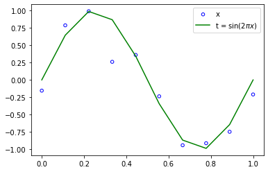
3. The data for this example is generated from the function
   $f(x) = \sin(2\pi x)$ + Gaussian distribution random noise

4. $X = (x_1,...,x_N)^T \\t = (t_1,...,t_N)^T \\ N=10 [0,1]$

5. new predict value = $\hat y$
   new input value = $\hat x$
   

Solution

polynomial function
$y(x,w) = w_0 + w_1x + w_2x^2 + ... + w_Mx^M =\displaystyle\sum_{j=0}^{M}{(w_jx^i)}$
polynomial coefficients : $w$

1. Polynomial Regression

Section 1.5 에서 자세히

Error minimize
$E(w)=\frac{1}{2}\displaystyle\sum_{n=1}^{N}({y(x_n,w)-t_n})^2$

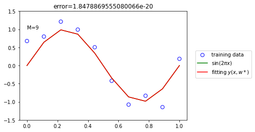
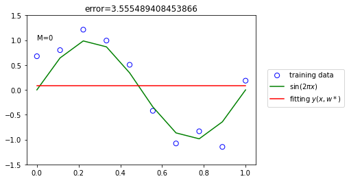
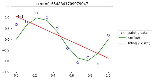
The resulting polynomial is given by the function $y(x,w^*)$
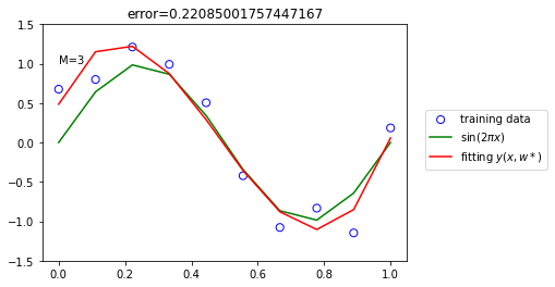
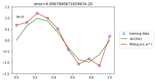
There remains the problem of choosing the order M of the polynomial M = 0,1,3 and 9.

Replace with Moore-Penrose 유사 역행렬
출처
http://matrix.skku.ac.kr/math4ai-intro/W5/
https://deep-learning-study.tistory.com/482
https://pasus.tistory.com/31

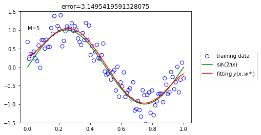
Model fit : $W=X^{+} \times Y$
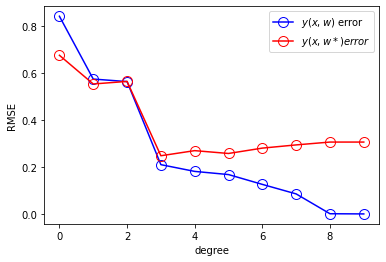
Model predict : $Y=X \times W$

Training

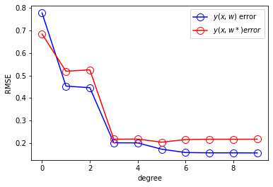
RMSE 비교

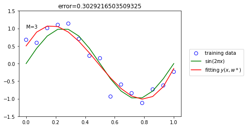
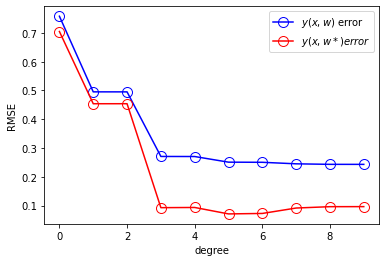
N 증가 비교
N = 15

N = 100

One technique that is oftenused to control the over-fitting phenomenon in such cases is that of regularization,which involves adding a penalty term to the error function in order to discouragethe coefficients from reaching large values. The simplest such penalty term takes theform of a sum of squares of all of the coefficients, leading to a modified error functionof the form

2. Regularization Regression (Ridge Regression)

Section 5.5 에서 자세히
https://sanghyu.tistory.com/13

평균제곱오차를 최소화하는 회귀계수($\beta=(\beta_1,...,\beta_p)$) 계산

$\hat B^{LS} = \argmin MSE = (X^TX)^{-1}X^TY$

회귀계수 $\beta$ 에대한 unbiased estimator 중 가장 분산이 작은 estimator
(Best Linear Unbiased Estimarot : BLUE, Gauss-Markov Theorem)

위 선형회귀 식(polynomial function)에 L2 normalization 항 추가
$W^*=\argmin|t-XW| + \alpha||W||^2$
$||w||^2=w^Tw=w_o$

Solve
$\\Ax=B$
$A=\alpha * I +X^TX$
$B=X^TY$

$Predict\\\hat t=xw^*$