ML) Credit Card Fraud Detection - LogisticRegression / DecisionTreeClassifier / RandomForestClassifier / LGBMClassifier

1. 데이터 가져오기
import pandas as pd

data_path = '.../data/Credit Card Fraud Detection.csv'
raw_data = pd.read_csv(data_path)

raw_data.columns
# 결과 :
Index(['Time', 'V1', 'V2', 'V3', 'V4', 'V5', 'V6', 'V7', 'V8', 'V9', 'V10',
       'V11', 'V12', 'V13', 'V14', 'V15', 'V16', 'V17', 'V18', 'V19', 'V20',
       'V21', 'V22', 'V23', 'V24', 'V25', 'V26', 'V27', 'V28', 'Amount',
       'Class'],
      dtype='object')
2. 데이터 확인
import seaborn as sns
import matplotlib.pyplot as plt

sns.countplot(x='Class', data=raw_data)
plt.show()
# 결과 : 아래 그래프 이미지

X = raw_data.iloc[:, 1:-1]
y = raw_data.iloc[:, -1]

X.shape, y.shape
# 결과 :
((284807, 29), (284807,))
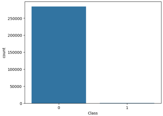
3. Train & Test Split (1)
from sklearn.model_selection import train_test_split

X_train, X_test, y_train, y_test = train_test_split(X, y, test_size=0.3, stratify = y, random_state=4)
4. 모델 평가 함수 생성
from sklearn.metrics import (accuracy_score, precision_score, recall_score, f1_score, roc_auc_score)
from sklearn.metrics import confusion_matrix

# 평가 점수를 계산하는 가장 기본 함수

def get_clf_eval(y_test, pred):
  acc = accuracy_score(y_test, pred)
  pre = precision_score(y_test, pred)
  re = recall_score(y_test,pred)
  f1 = f1_score(y_test, pred)
  auc = roc_auc_score(y_test, pred)

  return [acc, pre, re, f1, auc]


# 평가 점수와 혼동 행렬 출력

def print_clf_eval(y_test, pred):

  acc, pre, re, f1, auc = get_clf_eval(y_test, pred)
  confusion = confusion_matrix(y_test, pred)

  print('==> confusion matrix')
  print(confusion)
  print('====================')
  print(f'accuracy: {acc:.4f}, precision: {pre:.4f}')
  print(f'recall: {re:.4f}, f1: {f1:.4f}, auc: {auc:.4f}')


# 단일 모델의 학습, 예측, 평가.

def get_result(model, X_train, X_test,y_train, y_test):

  model.fit(X_train, y_train)
  pred = model.predict(X_test)

  return get_clf_eval(y_test, pred)


# 여러 모델 평가 결과를 DataFrame으로 반환

def get_result_pd(models, model_names, X_train, X_test, y_train, y_test):

  col_names = ['accuracy', 'precision', 'recall', 'f1', 'roc_auc']
  tmp = []

  for model in models:
    tmp.append(get_result(model, X_train, X_test, y_train, y_test))

  return pd.DataFrame(tmp, columns=col_names, index=model_names)
5. LogisticRegression 적용
from sklearn.linear_model import LogisticRegression

lr_clf = LogisticRegression(solver='liblinear', random_state=4)
lr_clf.fit(X_train, y_train)
lr_pred = lr_clf.predict(X_test)

print_clf_eval(y_test, lr_pred)
# 결과
==> confusion matrix
[[85275    20]
 [   42   106]]
====================
accuracy: 0.9993, precision: 0.8413
recall: 0.7162, f1: 0.7737, auc: 0.8580
6. DecisionTreeClassifier 적용
from sklearn.tree import DecisionTreeClassifier

dt_clf = DecisionTreeClassifier(max_depth=4, random_state=4)
dt_clf.fit(X_train, y_train)
dt_pred = dt_clf.predict(X_test)

print_clf_eval(y_test, dt_pred)
# 결과
==> confusion matrix
[[85271    24]
 [   30   118]]
====================
accuracy: 0.9994, precision: 0.8310
recall: 0.7973, f1: 0.8138, auc: 0.8985
7. RandomForestClassifier 적용
from sklearn.ensemble import RandomForestClassifier

rf_clf = RandomForestClassifier(n_estimators=100, random_state=4)
rf_clf.fit(X_train, y_train)
rf_pred = rf_clf.predict(X_test)

print_clf_eval(y_test, rf_pred)
# 결과 :
==> confusion matrix
[[85287     8]
 [   32   116]]
====================
accuracy: 0.9995, precision: 0.9355
recall: 0.7838, f1: 0.8529, auc: 0.8918
8. LGBMClassifier 적용
!pip install lightgbm
from lightgbm import LGBMClassifier

lgbm_clf = LGBMClassifier(random_state=4, n_estimators=1000, num_liaves=64, boost_from_average=False)
lgbm_clf.fit(X_train, y_train)
lgbm_clf_pred = lgbm_clf.predict(X_test)

print_clf_eval(y_test, lgbm_clf_pred)
# 결과 :
==> confusion matrix
[[85290     5]
 [   29   119]]
====================
accuracy: 0.9996, precision: 0.9597
recall: 0.8041, f1: 0.8750, auc: 0.9020
9. 각 모델별 결과 DataFrame 생성 (1)
models = [lr_clf, dt_clf, rf_clf, lgbm_clf]
model_names = ['LogisticReg', 'DecisionTree', 'RandomForest', 'LightGBM']

results = get_result_pd(models, model_names, X_train, X_test, y_train, y_test)
results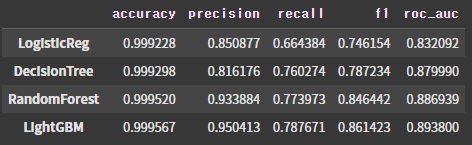
10. Amount열 - 시각화 (이상치 열 확인)
plt.figure(figsize=(8,4))
sns.histplot(raw_data['Amount'], color='r', kde=True)
plt.ylim(0, 20000)
plt.show()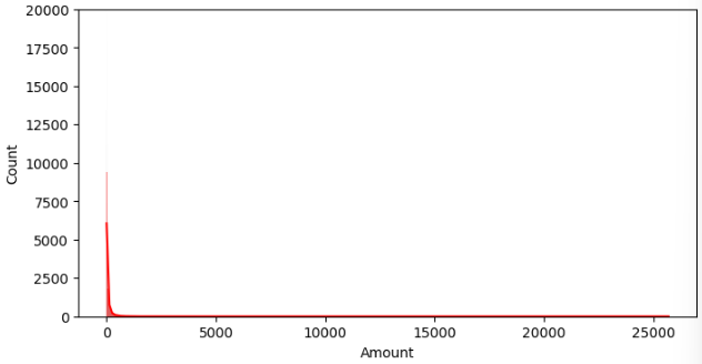
11. Amount열 - Standard Scaler 적용
from sklearn.preprocessing import StandardScaler

# 표준화
scaler = StandardScaler()
amount_n = scaler.fit_transform(raw_data['Amount'].values.reshape(-1,1))

# 원래 Amount 열 제거 -> Scaling한 열 추가
raw_data_copy = raw_data.iloc[:, 1:-2]
raw_data_copy['Amount_Scaled'] = amount_n
raw_data_copy.head()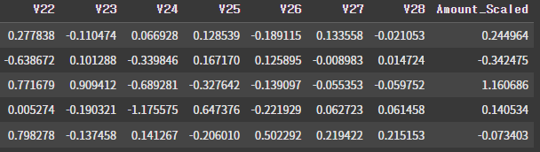
12. Train & Test Re-Split (2)
# 누락되어 있는 듯
X = raw_data_copy

X_train, X_test, y_train, y_test = train_test_split(X, y, test_size=0.3, stratify=y, random_state=4)
13. 각 모델별 결과 DataFrame 생성 (2)
models = [lr_clf, dt_clf, rf_clf, lgbm_clf]
model_names = ['LogisticReg', 'DecisionTree', 'RandomForest', 'LightGBM']

results = get_result_pd(models, model_names,  X_train, X_test, y_train, y_test)
results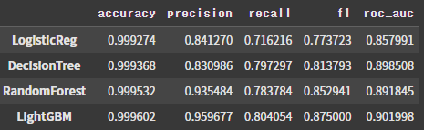
14. Amount열 - 로그 변환
- 로그 변환은 일반적으로 데이터의 스케일을 줄이고 분포를 정규화(또는 비슷하게)하는 데 사용
- 큰 값의 영향을 줄이고, 상대적으로 작은 값들의 중요도를 높임
- 데이터의 분포를 더 균일하게 만들어 모델의 성능을 향상
import numpy as np

amount_log = np.log1p(raw_data['Amount'])

# Standard Scaling 했었던 Amount_Scaled열을 로그 변환으로 변경
raw_data_copy['Amount_Scaled'] = amount_log
15. Amount열 - 로그 변환 결과 시각화
plt.figure(figsize=(8,4))
sns.histplot(raw_data_copy['Amount_Scaled'], color='r', kde=True)
plt.show()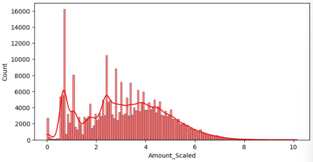
16. Train & Test Re-Split (3)
X = raw_data_copy

X_train, X_test, y_train, y_test = train_test_split(X, y, test_size=0.3, stratify=y, random_state=4)
17. 각 모델별 결과 DataFrame 생성 (3)
models = [lr_clf, dt_clf, rf_clf, lgbm_clf]
model_names = ['LogisticReg', 'DecisionTree', 'RandomForest', 'LightGBM']

results = get_result_pd(models, model_names, X_train, X_test, y_train, y_test)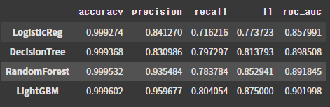
18. V13, 14, 15열 - 시각화 (이상치 열 확인)
plt.figure(figsize=(8,4))
sns.boxplot(data=raw_data[['V13', 'V14', 'V15']])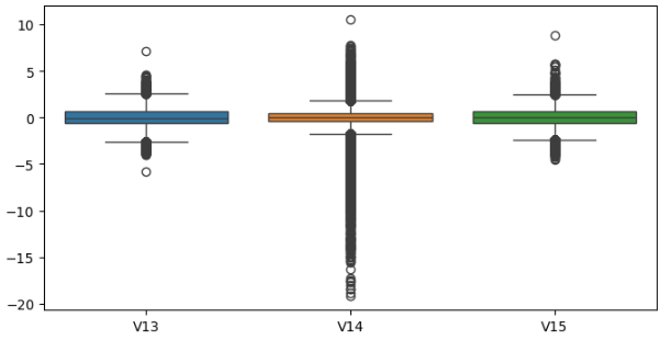
19. Outlier 탐지 함수 생성
def get_outlier(df=None, column=None, weight=1.5):
  fraud = df[df['Class']==1][column]

  quantile_25 = np.percentile(fraud.values, 25)
  quantile_75 = np.percentile(fraud.values, 75)
  iqr = quantile_75 - quantile_25

  iqr_weight = iqr * weight
  lowest_val = quantile_25 - iqr_weight
  highest_val = quantile_75 + iqr_weight

  outlier_index = fraud[(fraud < lowest_val) | (fraud > highest_val)].index
  return outlier_index

get_outlier(df=raw_data, column='V14')
# 결과 :
Index([8296, 8615, 9035, 9252], dtype='int64')
20. Outlier 제거
# 데이터의 shape
raw_data_copy.shape
# 결과 :
(284807, 29)

outlier_index = get_outlier(df=raw_data, column='V14')

# 이상치 제거
raw_data_copy.drop(outlier_index, axis=0, inplace=True)
raw_data_copy.shape
# 결과 :
(284803, 29)
21. Train & Test Re-Split (4)
- 레이블 (타겟 변수)에는 outlier 제거 및 scaling 불필요
- Outlier 제거 및 Scaling은 feature(독립 변수)의 범위를 조정해 모델 학습을 돕는 것이 목적
X = raw_data_copy

raw_data.drop(outlier_index, axis=0, inplace=True)

y = raw_data.iloc[:,-1]

X_train, X_test, y_train, y_test = train_test_split(X, y, test_size=0.3, stratify=y, random_state=4)

models = [lr_clf, dt_clf, rf_clf, lgbm_clf]
model_names = ['LogisticReg', 'DecisionTree', 'RandomForest', 'LightGBM']

results = get_result_pd(models, model_names, X_train, X_test, y_train, y_test)
results 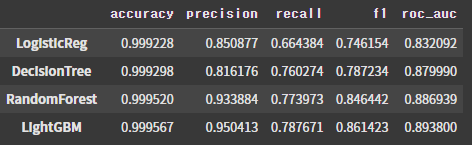
22. SMOTE
- 불균형한 데이터셋에서 소수 클래스의 샘플을 생성하여 클래스 균형을 맞추는 오버샘플링 기법
- 실제 데이터를 복제하지 않고, 소수 클래스 샘플의 특징을 바탕으로 새로운 데이터를 생성
X_train.shape, y_train.shape
# 결과 :
((199362, 29), (199362,))

np.unique(y_train, return_counts=True)
# 결과 : 클래스 불균형이 심각 / 클래스 1의 샘플 수가 클래스 0에 비해 매우 적음
(array([0, 1]), array([199020,    342]))

from imblearn.over_sampling import SMOTE

smote = SMOTE(random_state=4)

# 오버샘플링된 데이터셋 반환
X_train_over, y_train_over = smote.fit_resample(X_train, y_train)

np.unique(y_train_over, return_counts=True)
# 결과 (클래스 값 / 샘플 수):
(array([0, 1]), array([199020, 199020]))
23. 각 모델별 결과 DataFrame 생성 (4)
models = [lr_clf, dt_clf, rf_clf, lgbm_clf]
model_names = ['LogisticReg', 'DecisionTree', 'RandomForest', 'LightGBM']

results = get_result_pd(models, model_names, X_train_over, X_test, y_train_over, y_test)
results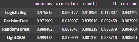

Perfect timing to be a Newbie