Hands-On Marchine Learning w/Scikit-Learn & TensorFlow - 3. Classification [MNIST]

# 데이터 불러오기, 확인하기 
from sklearn.datasets import fetch_openml
mnist = fetch_openml('mnist_784', version=1)
mnist.keys()
# 결과 : dict_keys(['data', 'target', 'frame', 'categories', 'feature_names', 'target_names', 'DESCR', 'details', 'url'])

# X.shape는 X 데이터의 크기(행과 열 수)를 반환
# 70000: 총 70,000개의 이미지가 포함되어 있음을 의미
# 784: 각 이미지가 784개의 픽셀 특징을 가진 벡터로 변환되어 있음을 의미 (28x28 픽셀 이미지를 1차원으로 펼친 것)
# y.shape = (70000,)는 벡터 형태로, 1차원 배열
X, y = mnist['data'], mnist['target']
print(X.shape) # 결과 : (70000, 784)
print(y.shape) # 결과 : (70000,)

import matplotlib as mpl
import matplotlib.pyplot as plt

some_digit = X.iloc[0].to_numpy()
some_digit_image = some_digit.reshape(28,28)

plt.imshow(some_digit_image, cmap=mpl.cm.binary, interpolation='nearest')
plt.axis('off')
plt.show()

y[0] # 결과: '5'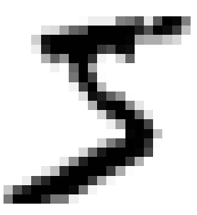

import numpy as np

# 숫자 라벨이 0에서 255 범위 안에 있을 때 메모리 효율적으로 저장하기에 유용
y = y.astype(np.uint8)

# train, test셋 나누기 
X_train, X_test, y_train, y_test = X[:60000], X[60000:], y[:60000], y[60000:]

# 이진 레이블 생성 (True / False)
y_train_5 = (y_train == 5) # True
y_test_5 = (y_test == 5) # True

from sklearn.linear_model > import SGDClassifier

• SGDClassifier는 scikit-learn에서 제공하는 확률적 경사 하강법(Stochastic Gradient Descent) 기반의 분류 모델
• 데이터의 일부(배치)를 사용해 모델을 업데이트하는 확률적 경사 하강법 사용. 전체 데이터를 사용하는 경사 하강법보다 빠르게 수렴하며, 특히 대규모 데이터셋에서 메모리 효율적.
• 온라인 학습(한 번에 한 데이터 포인트씩 학습)에 적합
• SGDClassifier는 선형 모델로 작동하고 Logistic Regression이나 SVM (Support Vector Machine) 같은 선형 모델의 학습에 사용
• loss 파라미터를 통해 사용할 손실 함수를 지정할 수 있음

# Stochastic Gradient Descent classifier를 사용해 숫자 5를 감지하는 이진 분류 모델을 학습하고, some_digit이 숫자 5인지 예측
from sklearn.linear_model import SGDClassifier

# SGDClassifier의 인스턴스를 생성
sgd_clf = SGDClassifier(random_state=42)

# 학습 데이터(X_train)와 이진 레이블(y_train_5)을 사용하여 모델을 학습
# 이진 레이블 y_train_5는 숫자가 5일 때 True, 그렇지 않을 때 False로 설정되어 있음
sgd_clf.fit(X_train, y_train_5)

# some_digit이 5인지 예측
sgd_clf.predict([some_digit]) # 결과: array([ True])

from sklearn.model_selection > import cross_val_score

• cross_val_score를 사용해 SGDClassifier의 교차 검증 성능을 평가
• 3-폴드 교차 검증을 수행하고, 모델의 정확도(accuracy)를 측정
• 불균형 데이터(non 5 : 90%)에서 모델이 주로 다수 클래스에만 집중할 경우 정확도가 떨어지는 문제점
• 불균형 데이터에서는 precision, recall이 더 유용한 평가 지표

# cross_val_score 함수는 데이터를 여러 폴드로 나누어 교차 검증을 수행하며, 각 폴드의 성능을 측정
from sklearn.model_selection import cross_val_score

cross_val_score(sgd_clf, X_train, y_train_5, cv=3, scoring='accuracy')
# 결과 : array([0.95035, 0.96035, 0.9604 ])

from sklearn.model_selection > import cross_val_predict

from sklearn.metrics import > confusion_matrix

• cross_val_predict를 사용해 예측값을 생성하고, confusion_matrix를 통해 예측 결과와 실제 레이블 간의 혼동 행렬(Confusion Matrix)을 계산
• cross_val_score(각 폴드에서 모델이 얼마나 잘 예측했는지 점수로 평가)와 달리 cross_val_predict는 각 폴드에서 훈련된 모델로 예측한 결과(예측값)를 반환

from sklearn.model_selection import cross_val_predict

# y_train_pred : 교차 검증을 통해 얻어진 예측값을 저장. 각 데이터 포인트에 대한 True 또는 False 예측값 포함
y_train_pred = cross_val_predict(sgd_clf, X_train, y_train_5, cv=3)
 
from sklearn.metrics import confusion_matrix

# y_train_5: 실제 레이블. 숫자 5인 경우 True, 그렇지 않은 경우 False.
# y_train_pred: 모델이 예측한 레이블.
confusion_matrix(y_train_5, y_train_pred)

# 결과 : array([[53892,   687],
      		   [ 1891,  3530]], dtype=int64)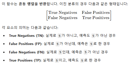

from sklearn.metrics import > precision_score, recall_score

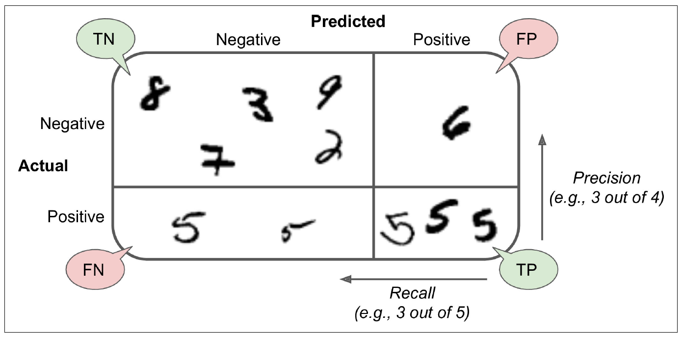
• scikit-learn의 metrics 모듈에서 precision, recall을 계산하는 precision_score와 recall_score 함수
• 이 두 함수는 이진 분류 및 다중 클래스 분류에서 각각의 정밀도와 재현율을 계산하는 데 사용
• precision : 양성으로 예측한 것 중에서 실제로 양성인 비율을 의미
• recall : 실제 양성인 것 중에서 모델이 양성으로 예측한 비율

from sklearn.metrics import precision_score, recall_score

print(precision_score(y_train_5, y_train_pred))
print(recall_score(y_train_5, y_train_pred))

# 결과 
0.8370879772350012
0.6511713705958311

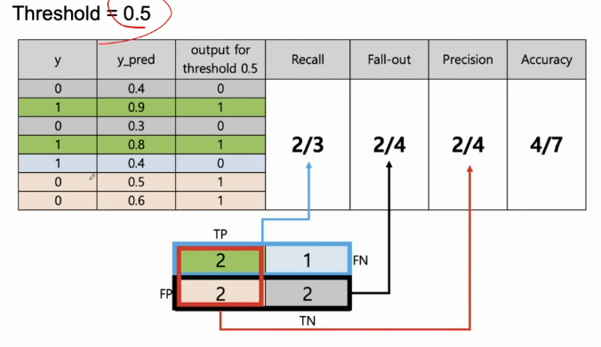
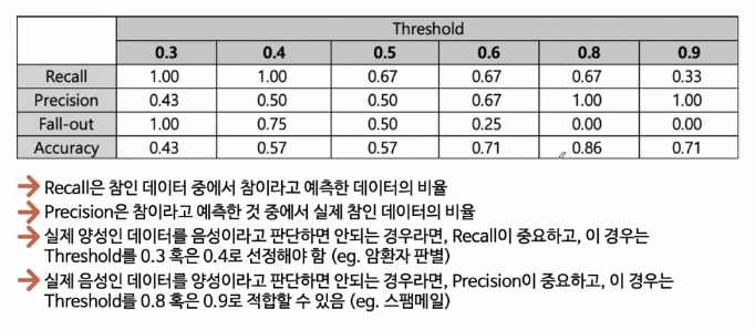
• Accuracy : 전체 중에 맞춘것
• Recall : 실제 1 중에 1이라고 맞춘 것
• Fall-out : 실제 0 중에 0이라고 맞춘 것
• Precision : 1이라고 예측한 것 중 1인 것

from sklearn.metrics > import f1_score

• 모델의 F1 점수를 계산
• F1 점수는 precision, recall의 조화 평균
• precision, recall이 모두 높을 때 높은 값을 가ㅈ고, 한쪽이 낮아지면 F1 점수도 낮아짐 (낮은 곳에 더 큰 가중치)
• 특히 불균형 데이터에서 모델의 성능을 평가할 때 유용

from sklearn.metrics import f1_score

f1_score(y_train_5, y_train_pred)
# 결과 : 0.7325171197343847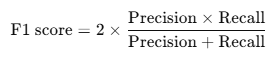

* - decision_function

• SGDClassifier의 메서드로, 각 샘플에 대해 예측할 때 결정 점수(decision score)를 계산하고 반환
• decision score는 모델이 특정 클래스(예: 숫자 5)에 속할 가능성에 대한 확신 정도를 수치로 나타냄. 양수일수록 양성 클래스(ex. 숫자 5)로 분류할 가능성이 높고, 음수일수록 음성 클래스일 가능성이 높음
• 이를 threshold와 비교하여 최종적으로 예측 클래스를 결정
• 일반적으로 threshold는 0으로 설정. 즉, decision score가 0보다 크면 양성(True), 0보다 작으면 음성(False)으로 예측하는 방식
• 이 threshold를 조정하면 precision과 recall의 균형이 달라짐.
• 높은 threshold: 더 확실한 경우에만 양성으로 예측하므로 precision이 높아지는 대신 recall이 낮아짐
• 낮은 threshold: 예측에 더 관대해지므로 recall이 높아지는 대신 precision이 낮아질 수 있습니다.

# 교차 검증 없이 이미 학습된 모델로 단일 샘플에 대한 decision score를 즉시 계산하는 예시 
# [some_digit] : decision_function은 입력을 2차원 배열로 받음 
y_scores = sgd_clf.decision_function([some_digit])
y_scores

# threshold: 예측을 양성(True) 또는 음성(False)으로 나누는 기준점
# SGDClassifier는 0으로 threshold 기본값 설정 (이전과 결과 동일) 
threshold=0

# y_scores가 threshold보다 큰지 비교하여 True 또는 False 값을 반환
# decision score가 임계값보다 크다면 True(즉, 5로 예측)로 반환
y_some_digit_pred = (y_scores > threshold)
y_some_digit_pred # 결과 : array([ True])

# theshold를 높이면 recall이 낮아짐 
threshold = 8000
y_some_digit_pred = (y_scores > threshold)
y_some_digit_pred # 결과 : array([False])

from sklearn.metrics > import precision_recall_curve

• Precision-Recall Curve를 그리기 위해 필요한 값들을 계산
• precision_recall_curve를 사용해 precision, recall, threshold 값을 계산하고, 이 값을 바탕으로 precision, recall값을 threshold에 대해 시각화
• 이 함수는 threshold를 조정하면서 precision, recall이 어떻게 변화하는지 파악할 때 유용

# 교차 검증을 수행해 각 데이터 포인트에 대한 예측값을 반환
# 보통 cross_val_predict는 예측된 클래스(예: True 또는 False)를 반환하지만, method 인자를 설정하면 decision score 또는 확률값과 같은 추가적인 예측 정보를 반환
# sgd_clf: 예측에 사용할 classifier (SGDClassifier의 객체)
# method='decision_function': cross_val_predict에 method='decision_function'을 추가하여, 예측 클래스가 아닌 결정 점수(decision score)를 반환하도록 설정
y_scores = cross_val_predict(sgd_clf, X_train, y_train_5, cv=3, method='decision_function')

from sklearn.metrics import precision_recall_curve

# precision_recall_curve: 이 함수는 실제 레이블과 결정 점수를 사용해 precisions, recalls, thresholds 값을 계산
# 결과값들은 배열로 나옴 
precisions, recalls, thresholds = precision_recall_curve(y_train_5, y_scores)

# precision, recall을 threshold에 대해 시각화하는 함수
def plot_precision_recall_vs_threshold(precisions, recalls, thresholds):
    # precisions[:-1]: y축에 정밀도를 표시. precision_recall_curve는 thresholds 배열의 길이보다 하나 더 많은 정밀도 값을 반환하기 때문에, 마지막 요소를 제외한 값만 사용
    # 'b--': 파란색 점선
    plt.plot(thresholds, precisions[:-1], 'b--', label='Precision')
    plt.plot(thresholds, recalls[:-1], 'g-', label='Recall')

     # 특정 threshold 값 강조
    threshold_important = 8000
    precision_important = precisions[np.argmax(thresholds >= threshold_important)]
    recall_important = recalls[np.argmax(thresholds >= threshold_important)]

    # 세로 점선
    plt.plot([threshold_important, threshold_important], [0, precision_important], "r:")
    # 빨간 점 (precision, recall)
    plt.plot([threshold_important], [precision_important], "ro")
    plt.plot([threshold_important], [recall_important], "ro")
    plt.plot([threshold_important, threshold_important], [precision_important, recall_important], "r:")

    # 가로 점선 추가
    plt.plot([-50000, threshold_important], [precision_important, precision_important], "r:")
    plt.plot([-50000, threshold_important], [recall_important, recall_important], "r:")

    # x축 범위 설정 및 그리드 추가
    plt.xlim(-50000, 50000)
    plt.grid(True)

    plt.xlabel("Threshold")
    plt.legend(loc="best")
    plt.ylim([0, 1])

plot_precision_recall_vs_threshold(precisions, recalls, thresholds)
plt.show()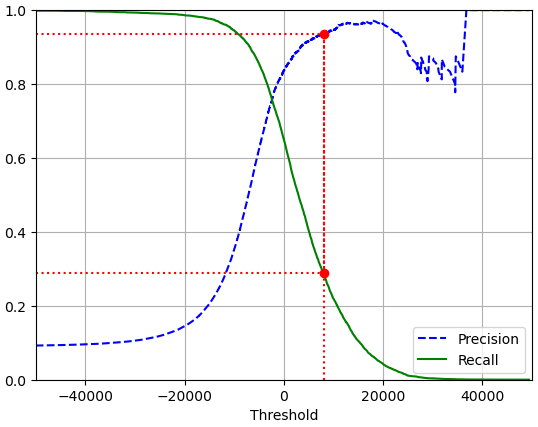

precision > 0.9

• precision이 0.9 이상이 되도록 설정한 특정 threshold에서의 예측 결과를 계산하고, 그에 따른 precision과 recall을 출력

# precisions >= 0.9 : precision이 0.9 이상인 위치를 True로 반환하는 불리언 배열을 생성
# np.argmax : 이 불리언 배열에서 True가 처음 나타나는 인덱스를 반환
# 이 인덱스를 통해 precision이 0.9 이상이 되는 첫 번째 threshold 값 확보 
threshold_90_precision = thresholds[np.argmax(precisions >= 0.9)]

# decision score(y_scores)가 threshold_90_precision 이상일 때 True, 그렇지 않을 때 False로 예측값을 생성
# y_train_pred_90 : precision이 0.9 이상이 되는 threshold에서 양성(True)으로 예측된 샘플들 표시
y_train_pred_90 = (y_scores >= threshold_90_precision)

# precision, recall 값 계산 

precision_score(y_train_5, y_train_pred_90) # 결과 : 0.9000345901072293
recall_score(y_train_5, y_train_pred_90) # 결과 : 0.4799852425751706

from sklearn.metrics > import roc_curve

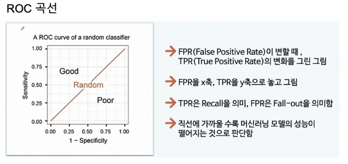
• roc_curve 함수는 ROC 곡선을 그리는 데 필요한 값들을 계산
• ROC 곡선은 주로 이진 분류 모델의 성능을 평가하는 데 사용
• tpr과 fpr의 관계를 threshold에 따라 보여줌
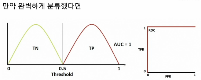
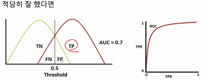
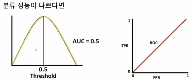
• ROC 곡선의 AUC(Area Under Curve)는 모델의 전반적인 성능을 나타내는 지표로, 값이 클수록 성능이 좋음
• fpr (False Positive Rate) : fpr은 음성 샘플 중에서 잘못 양성으로 예측된 비율을 의미
  
• tpr (True Positive Rate) : 실제 양성 샘플 중에서 양성으로 정확히 예측된 비율 (=recall)
  
• threshold : 각 임계값에서 fpr과 tpr을 계산하는 데 사용된 threshold 값. threshold를 조정하면서 fpr과 tpr의 변화를 확인

from sklearn.metrics import roc_curve

fpr, tpr, thresholds = roc_curve(y_train_5, y_scores)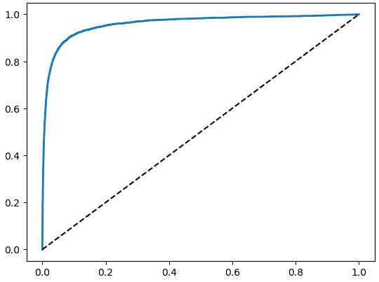

from sklearn.metrics > import roc_auc_score

• roc_auc_score는 scikit-learn의 metrics 모듈에 포함된 함수로, ROC 곡선의 AUC (Area Under the Curve) 점수를 계산
• AUC 점수는 모델이 양성 클래스와 음성 클래스를 얼마나 잘 구분하는지 평가하는 지표
• 1에 가까울수록 좋은 성능을 의미하고, 0.5는 무작위 예측과 같은 성능
• 예를 들어, AUC가 0.9라면 양성 클래스와 음성 클래스를 높은 정확도로 구분할 수 있다는 것을 의미

from sklearn.metrics import roc_auc_score

# y_train_5: 실제 레이블. 양성(True)과 음성(False)을 포함하는 이진 벡터
# y_scores: 모델의 decision score 또는 예측 확률. 각 샘플이 양성 클래스(예: 숫자 5)일 가능성을 수치로 나타냄 
roc_auc_score(y_train_5, y_scores) # 결과 : 0.9604938554008616

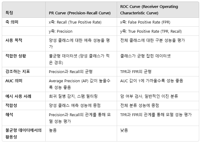
* - PR Curve vs. ROC Curve

• PR Curve는 양성 클래스의 예측 성능을 강조하기 때문에, 불균형 데이터에서 특히 유용
• ROC Curve는 전체적인 양성/음성 분류 성능을 나타내며, 클래스가 균형 잡힌 데이터셋에서 더 적합
• 불균형 데이터에서는 ROC Curve의 AUC가 높은 경우에도 precision이 낮아 실제 성능이 부정확할 수 있으므로, 이 경우에는 PR Curve를 보는 것이 더 적절

Multiclass Classification

• SGDClassifier를 사용하여 some_digit에 대한 예측 결과를 확인하고, 모델의 결정 점수, 클래스 목록, 그리고 특정 인덱스의 클래스를 확인

# SGDClassifier 모델을 학습 데이터(X_train, y_train)로 훈련
# y_train이 다중 클래스 레이블이라면, SGDClassifier는 OvA (One-vs-All) 방식으로 각 클래스를 분류할 수 있도록 모델을 학습
sgd_clf.fit(X_train, y_train)

# some_digit이 어떤 클래스(숫자)로 예측되는지 확인
# 출력값은 모델이 예측한 클래스의 레이블(예: 3, 5, 9 등)을 반환
sgd_clf.predict([some_digit]) # 결과 : array([3], dtype=uint8)


# decision_function을 사용해 some_digit에 대한 각 클래스별 decision score를 계산
some_digit_scores = sgd_clf.decision_function([some_digit])
some_digit_scores 
# 결과 
array([[-31893.03095419, -34419.69069632,  -9530.63950739,
          1823.73154031, -22320.14822878,  -1385.80478895,
        -26188.91070951, -16147.51323997,  -4604.35491274,
        -12050.767298  ]])

# 가장 큰 값의 인덱스를 반환
np.argmax(some_digit_scores) # 결과 : 3

# SGDClassifier가 학습한 모든 클래스 레이블을 담고 있는 배열
sgd_clf.classes_ # 결과 : array([0, 1, 2, 3, 4, 5, 6, 7, 8, 9], dtype=uint8)

# sgd_clf.classes_ 배열에서 인덱스 3에 해당하는 클래스를 반환
sgd_clf.classes_[3] # 결과 : 3

from sklearn.multiclass > import OneVsOneClassifier

• OneVsOneClassifier : 주어진 기본 분류기(base classifier)를 사용하여 모든 클래스 쌍에 대해 개별적인 이진 분류기를 학습
• 여기서는 SGDClassifier를 기본 분류기로 설정하여 각 클래스 쌍을 구분하는 이진 분류기를 학습

from sklearn.multiclass import OneVsOneClassifier

# SGDClassifier를 OvO 방식으로 다중 클래스 분류에 사용하도록 설정
ovo_clf = OneVsOneClassifier(SGDClassifier(random_state=42))

# X_train과 y_train을 사용해 ovo_clf 모델을 학습
ovo_clf.fit(X_train, y_train)

# some_digit에 대해 예측을 수행
ovo_clf.predict([some_digit])

# ovo_clf.estimators_ : 모든 클래스 쌍에 대해 학습된 이진 분류기들이 저장되어 있음
# OvO 방식으로 생성된 이진 분류기의 수를 반환
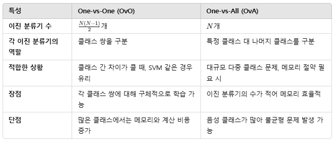
len(ovo_clf.estimators) # 결과 : 45 (10x9/2)

• OvO (one-versus-one) vs OvA (one-versus-all)
  : 클래스가 적고 클래스 간 구분이 명확하다면 OvO가 더 나은 선택
  : 대규모 데이터나 클래스가 많은 문제에서는 OvA가 더 효율적
  

from sklearn.ensemble > import RandomForestClassifier

• 여러 개의 결정 트리(Decision Tree)를 결합한 앙상블 학습 모델
• 랜덤 포레스트는 여러 결정 트리를 독립적으로 학습한 후, 모든 트리의 예측 결과를 투표 방식으로 결합하여 최종 예측
• RandomForestClassifier는 자체적으로 다중 클래스 분류를 처리할 수 있어, OvA나 OvO 기법이 필요하지 않음
• 과적합에 높은 성능, 노이즈에 민감한 결정 트리의 단점을 보완하여 더 높은 예측 정확도와 안정성을 제공

from sklearn.ensemble import RandomForestClassifier

# RandomForestClassifier 생성
forest_clf = RandomForestClassifier()

# RandomForestClassifier를 X_train과 y_train 데이터로 학습
forest_clf.fit(X_train, y_train)

# some_digit에 대해 예측을 수행
# RandomForestClassifier는 각 트리의 예측을 종합하여 최종 클래스를 결정하고, some_digit이 속할 가장 가능성이 높은 클래스를 예측
forest_clf.predict([some_digit])

# some_digit이 각 클래스에 속할 확률을 계산
# predict_proba 메서드 : 각 클래스에 대해 예측 확률을 반환하고, 이 확률들은 모두 합쳐서 1
forest_clf.predict_proba([some_digit])
# 결과 : array([[0.  , 0.01, 0.02, 0.11, 0.  , 0.86, 0.  , 0.  , 0.  , 0.  ]])

Cross Validation

• SGDClassifier의 accuracy 성능을 교차 검증으로 평가
• 정확도는 전체 예측 중에서 맞은 비율을 측정하지만, 불균형 데이터에서는 의미가 왜곡될 수 있음. 예를 들어, 특정 클래스가 매우 적은 경우, 모든 샘플을 다수 클래스로 예측하더라도 높은 정확도를 얻을 수 있음. 이 때는 precision, recall, 또는 f1-score와 같은 지표가 더 유용

# X_train: 학습에 사용할 입력 데이터
# y_train: 학습에 사용할 타겟 레이블
# scoring='accuracy': 모델 평가 지표
cross_val_score(sgd_clf, X_train, y_train, cv=3, scoring='accuracy')
# 결과 : array([0.87365, 0.85835, 0.8689 ])

from sklearn.preprocessing > import StandardScaler

• 데이터를 표준화하여 평균을 0, 표준편차를 1로 변환해 주는 전처리 도구
• 많은 머신러닝 알고리즘(특히 경사 하강법을 사용하는 모델)은 표준화된 데이터에서 더 안정적이고 빠르게 수렴하므로, 데이터를 표준화하는 것이 권장
• StandardScaler를 적용한 후 교차 검증 정확도가 더 높아질 가능성이 큼

from sklearn.preprocessing import StandardScaler

# StandardScaler의 인스턴스를 생성하여 scaler에 저장
# scaler 객체를 통해 데이터를 표준화할 수 있음 
scaler = StandardScaler()

# fit_transform 메서드를 사용하여 X_train 데이터를 표준화
# 연산 과정에서 데이터 타입 문제나 연산의 정확도가 떨어질 수 있기 때문에 실수형(float)으로 변환하여 사용하는 것이 더 안전
# X_train_scaled는 X_train의 각 특성이 평균 0, 표준편차 1로 변환된 표준화된 데이터
X_train_scaled = scaler.fit_transform(X_train.astype(np.float64))
cross_val_score(sgd_clf, X_train_scaled, y_train, cv=3, scoring='accuracy')
# 결과 array([0.8983, 0.891 , 0.9018]) = standard scale 이후 점수가 좀 더 높아짐

from sklearn.neighbors > import KNeighborsClassifier

• Multilabel Classification을 수행하기 위해 K-Nearest Neighbors (KNN) classifier를 사용
• KNN classifier는 가장 가까운 k개의 이웃을 기준으로 다수결을 통해 샘플의 클래스를 예측

from sklearn.neighbors import KNeighborsClassifier

# 첫 번째 레이블 생성 : y_train에서 7 이상인 경우를 True로, 7 미만인 경우를 False
y_train_large = (y_train >= 7)

# 두 번째 레이블 생성: y_train에서 홀수인 경우 True, 짝수인 경우 False
y_train_odd = (y_train % 2 ==1)

# y_multilabel의 각 행은 [y_train_large 값, y_train_odd 값] 형태로 두 개의 레이블을 포함
y_multilabel = np.c_[y_train_large, y_train_odd]

# KNN 인스턴스 생성 (k 기본값 : 5) 
knn_clf = KNeighborsClassifier()

# X_train과 다중 레이블 y_multilabel을 사용해 knn_clf 모델을 학습
knn_clf.fit(X_train, y_multilabel)

knn_clf.predict([some_digit])
# 결과 : array([[False,  True]])

# cross-validation을 통해 예측값을 반환
# knn_clf : 평가대상 = KNeighborsClassifier. 다중 레이블 분류를 수행할 수 있도록 y_multilabel에 대해 학습된 상태
# y_multilabel: 각 샘플에 대해 두 개의 레이블(7 이상 여부와 홀수 여부)을 포함하는 다중 레이블 벡터
# y_train_knn_pred : X_train의 각 샘플에 대해 예측된 다중 레이블 값이 저장됨
y_train_knn_pred = cross_val_predict(knn_clf, X_train, y_multilabel, cv=3)

# f1_score : 다중 레이블 예측에서 각 레이블의 F1 점수를 계산. F1 점수는 precision과 recall의 조화 평균으로, 모델의 예측 성능을 평가하는 데 유용
# average='macro' : 각 레이블에 대해 개별 F1 점수를 계산한 후, 모든 레이블에 동일한 가중치를 주어 평균을 계산
# macro 평균은 각 레이블의 중요도를 동일하게 가정하므로, 모든 레이블에 대해 고른 성능을 내는지 확인할 때 유용
# 출력값: f1_score의 결과는 y_multilabel과 y_train_knn_pred의 F1 점수를 나타내며, 이 값이 높을수록 모델이 두 레이블에 대해 높은 성능을 보였음을 의미
f1_score(y_multilabel, y_train_knn_pred, average='macro')
# 결과 : 0.9764102655606048