프로젝트 (Temp)
from sklearn.ensemble import RandomForestClassifier
from sklearn.model_selection import StratifiedKFold, GridSearchCV
from sklearn import metrics
import pandas as pd
import matplotlib.pyplot as plt
# Stratified K-Fold 설정
stratified_kfold = StratifiedKFold(n_splits=5, shuffle=True, random_state=13)
# 랜덤 포레스트 모델 초기화
model = RandomForestClassifier(random_state=13)
# 하이퍼파라미터 설정
param_grid = {
'n_estimators': [200, 300],
'max_depth': [30, 40],
'min_samples_split': [20, 30] ,
'min_samples_leaf': [6, 8] ,
'class_weight': ['balanced'],
'bootstrap': [True]
}
# GridSearchCV 초기화 (Stratified K-Fold 적용)
grid = GridSearchCV(
estimator=model,
param_grid=param_grid,
cv=stratified_kfold,
scoring='accuracy',
verbose=2,
return_train_score=True
)
# 데이터셋 학습
grid.fit(X_train, y_train)
# 최적의 하이퍼파라미터 출력
print("Best Parameters:", grid.best_params_)
print("Best Estimator:", grid.best_estimator_)
print("Best Score:", grid.best_score_)
# 테스트 데이터에 대한 예측 및 확률 출력
y_pred = grid.predict(X_test)
y_pred_proba = grid.predict_proba(X_test)[:, 1] # 클래스 1의 확률만 사용
# ROC Curve 계산
fpr, tpr, thresholds = metrics.roc_curve(y_test, y_pred_proba)
# AUC (Area Under Curve) 계산
roc_auc = metrics.auc(fpr, tpr)
# Classification Report 출력
print(metrics.classification_report(y_test, y_pred))
# Feature Importance 확인 (if applicable)
if hasattr(grid.best_estimator_, "feature_importances_"):
feature_importance = grid.best_estimator_.feature_importances_ # 특성 중요도
features = X_train.columns # 피처 이름
# 중요도와 피처를 정렬하여 출력
importance_df = pd.DataFrame({'Feature': features, 'Importance': feature_importance})
importance_df = importance_df.sort_values(by='Importance', ascending=False)
print(importance_df)
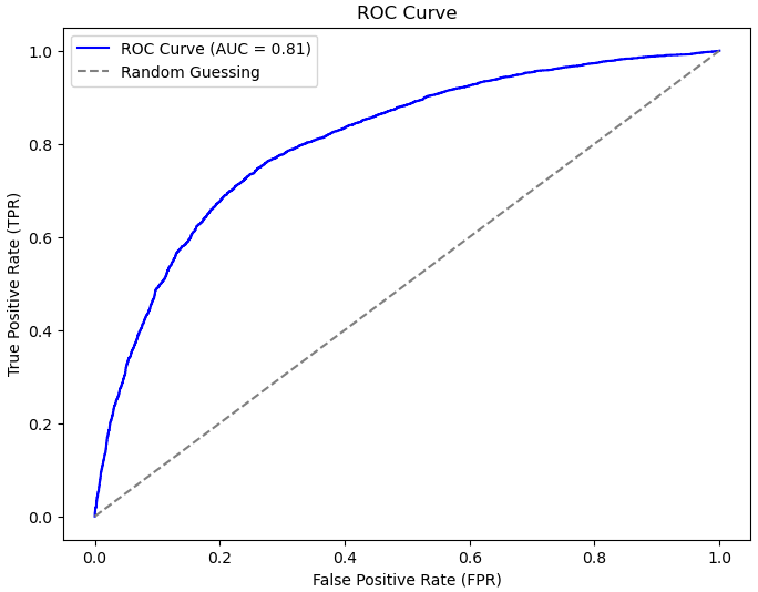
# ROC Curve 그리기
plt.figure(figsize=(8, 6))
plt.plot(fpr, tpr, color='blue', label=f'ROC Curve (AUC = {roc_auc:.2f})')
plt.plot([0, 1], [0, 1], linestyle='--', color='gray', label='Random Guessing')
plt.title('ROC Curve')
plt.xlabel('False Positive Rate (FPR)')
plt.ylabel('True Positive Rate (TPR)')
plt.legend()
plt.show()
# R :
Best Parameters: {'bootstrap': True, 'class_weight': 'balanced', 'max_depth': 30, 'min_samples_leaf': 6, 'min_samples_split': 30, 'n_estimators': 300}
Best Estimator: RandomForestClassifier(class_weight='balanced', max_depth=30,
min_samples_leaf=6, min_samples_split=30,
n_estimators=300, random_state=13)
Best Score: 0.7434302756860353
precision recall f1-score support
0 0.74 0.75 0.75 5759
1 0.74 0.73 0.74 5657
accuracy 0.74 11416
macro avg 0.74 0.74 0.74 11416
weighted avg 0.74 0.74 0.74 11416
Feature Importance
15 T/C_ratio 0.263799
9 Cont_length 0.258349
8 T_length 0.079925
7 STSB_SubCon_similarity 0.060529
10 SubT_length 0.057708
3 bait_top50_percentage 0.057563
6 STSB_TCon_similarity 0.057082
5 TFIDF_fam_Tword_score 0.045041
4 bait_top30_percentage 0.040793
12 TCon_cosine 0.020061
14 SubCon_cosine 0.015379
2 fam_word_score 0.013281
11 TCon_overlap 0.012910
13 SubCon_overlap 0.011645
16 special_char_cnt 0.002637
0 Q 0.001738
1 ! 0.001559
from sklearn.linear_model import LogisticRegression
from sklearn.model_selection import StratifiedKFold, GridSearchCV
from sklearn.preprocessing import MinMaxScaler
from sklearn import metrics
import pandas as pd
import matplotlib.pyplot as plt

# Stratified K-Fold 설정
stratified_kfold = StratifiedKFold(n_splits=5, shuffle=True, random_state=13)

# Logistic Regression 모델 초기화
model = LogisticRegression(random_state=13, solver='liblinear', max_iter=1000)

# 하이퍼파라미터 설정
param_grid = {
    'C': [0.0001, 0.001, 0.01],           # 규제 강도
    'penalty': ['l1', 'l2'],           # 정규화 (L1: Lasso, L2: Ridge)
    'class_weight': ['balanced', None] # 클래스 불균형 처리
}

# 데이터 스케일링 (Logistic Regression은 스케일에 민감함)
scaler = MinMaxScaler()
X_train_scaled = scaler.fit_transform(X_train)
X_test_scaled = scaler.transform(X_test)

# GridSearchCV 초기화 (Stratified K-Fold 적용)
grid = GridSearchCV(
    estimator=model,
    param_grid=param_grid,
    cv=stratified_kfold,
    scoring='accuracy',
    verbose=2,
    return_train_score=True
)

# 데이터셋 학습
grid.fit(X_train_scaled, y_train)

# 최적의 하이퍼파라미터 출력
print("Best Parameters:", grid.best_params_)
print("Best Estimator:", grid.best_estimator_)
print("Best Score:", grid.best_score_)

# 테스트 데이터에 대한 예측 및 확률 출력
y_pred = grid.best_estimator_.predict(X_test_scaled)
y_pred_proba = grid.best_estimator_.predict_proba(X_test_scaled)[:, 1]  # 클래스 1의 확률만 사용

# ROC Curve 계산
fpr, tpr, thresholds = metrics.roc_curve(y_test, y_pred_proba)

# AUC (Area Under Curve) 계산
roc_auc = metrics.auc(fpr, tpr)

# Classification Report 출력
print(metrics.classification_report(y_test, y_pred))

# ROC Curve 그리기
plt.figure(figsize=(8, 6))
plt.plot(fpr, tpr, color='blue', label=f'ROC Curve (AUC = {roc_auc:.2f})')
plt.plot([0, 1], [0, 1], linestyle='--', color='gray', label='Random Guessing')
plt.title('ROC Curve')
plt.xlabel('False Positive Rate (FPR)')
plt.ylabel('True Positive Rate (TPR)')
plt.legend()
plt.show()
import seaborn as sns
import matplotlib.pyplot as plt
import pandas as pd

# GridSearchCV 결과 가져오기
cv_results = pd.DataFrame(grid.cv_results_)

# 필요한 열만 추출 (C와 penalty 조합에 대한 mean test score)
pivot_table = cv_results.pivot_table(
    values='mean_test_score',
    index='param_C',
    columns='param_penalty'
)

# 히트맵 시각화
plt.figure(figsize=(8, 6))
sns.heatmap(pivot_table, annot=True, cmap='YlGnBu', fmt=".4f")
plt.title("Logistic Regression Grid Search Results")
plt.xlabel("Penalty")
plt.ylabel("C (Regularization Strength)")
plt.show()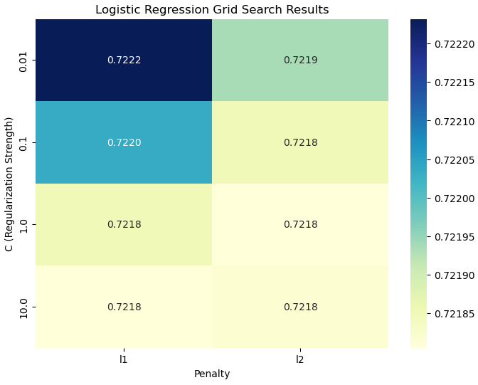

Perfect timing to be a Newbie